11 Day 11 (February 24)
11.1 Announcements
- Read Ch. 4 pgs 137-192
- You may also want to take a look at the notes we don’t get thru today.
- Concepts and Synthesis paper
- Questions/clarifications from journals
- “I am still struggling with non-identifiable parameters…”check out this book
- “What are your thoughts on just slapping location and year into the random effects and calling it a spatiotemporal model? We’ll be treating it as a starting point, but just curious of your thoughts?”
- “One thing I learned is that is that the most important thing is to write out the goals of your analyses. I don’t always think about it in this way. Sometimes I just have a dataset that I don’t have clear questions for, and so I ask myself what I could learn from this dataset, instead of starting with a goal/question.”
- “I am having trouble connecting the mathematical model we write on the board with what is happening in the R code when we simulate or fit the model”
- “I must admit that I have often used data from the closest weather station to my experiment sites. What are the risks of doing that, compared with using a statistical model to predict rainfall at the exact site?”
- “I am still struggling with non-identifiable parameters…”check out this book
11.2 Extreme precipitation in Kansas
Note, this is essentially the same as activity 2
On September 3, 2018 there was an extreme precipitation event that resulted in flooding in Manhattan, KS and the surrounding areas. If you would like to know more about this, check out this link and this video here and here.
My process
- Determine the goals of the study
- Data acquisition
- Live demonstration (Download R code here)
- Exploratory data analysis
- Live demonstration
- The model building process
- 1). Choose appropriate PDFs or PMFs for the data, process, and parameter models
- 2). Choose appropriate mathematical models for the “parameters” or moments of the PDFs/PMFs from step 1.
- 3). Choose an algorithm fit the statistical model to the data
- 4). Make statistical inference (e.g., calculate derived quantities and summarize the posterior distribution)
- Model checking, improvements, validation, and selection (Ch. 6)
What we will need to learn
- How to use R as a geographic information system
- New general tools from statistics
- Gaussian process
- Metropolis and Metropolis–Hastings algorithms
- Gibbs sampler
- How to use the hierarchical modeling framework to describe Kriging
- Hierarchical Bayesian model vs. “empirical” hierarchical model
- Specialized language used in spatial statistics (e.g., range, nugget, variogram)
11.3 Intro to GIS
- Spatio-temporal data from a statistical and GIS perspective are quite different
- Both disciplines, however, usually classify data based on the spatial support of the “data”
- Data from the GIS perspective
- Using R as a GIS, there are four main types of “data” that we will use.
- Shapefiles
- Raster
- Points
- Using R as a GIS, there are four main types of “data” that we will use.
11.3.1 Shapefiles
- Shapefiles are generally used to represent continuous spatial objects and boundaries
- Examples
- Rivers, streams, and lakes (e.g., National Hydrography Dataset)
- City of Manhattan (link)
- US Census (link)
- Example: Shapefiles of each state from the census website
library(sf)
library(sp)

download.file("http://www2.census.gov/geo/tiger/GENZ2015/shp/cb_2015_us_state_20m.zip",
    destfile = "states.zip")
unzip("states.zip")
sf.us <- st_read("cb_2015_us_state_20m.shp")
## Reading layer `cb_2015_us_state_20m' from data source
## `/Users/thefley/Library/CloudStorage/GoogleDrive-hefleyt2@gmail.com/My Drive/Teaching/Spring 2026/STAT 764 Lecture Notes (Spring 2026)/cb_2015_us_state_20m.shp'
## using driver `ESRI Shapefile'
## Simple feature collection with 52 features and 9 fields
## Geometry type: MULTIPOLYGON
## Dimension: XY
## Bounding box: xmin: -179.1743 ymin: 17.91377 xmax: 179.7739 ymax: 71.35256
## Geodetic CRS: NAD83sf.kansas <- sf.us[48, 6]
sf.kansas <- as(sf.kansas, "Spatial")
plot(sf.kansas, main = "", col = "white")
11.3.2 Raster
- Rasters are geographically referenced images (i.e., discrete spatial data)
- Examples
- PRSIM climate data (link)
- CropScape (link)
- National Elevation Dataset (link)
- National Land Cover Database (link)
- A few comments about raster files
- Raster files can be very large (e.g., NLCD is 1.1 Gb compressed and 18 Gb uncompressed)
- Raster “data” are usually model based predictions (e.g., PRISM) -Example: 2011 NLCD
library(raster)

# Large file that you may want to save on your computer
url.nlcd <- "https://www.dropbox.com/scl/fi/ew7yzm93aes7l8l37cn65/KS_2011_NLCD.img?rlkey=60ahyvxhq18gt0yr47tuq5fig&dl=1"
rl.nlcd2011 <- raster(url.nlcd)

plot(rl.nlcd2011)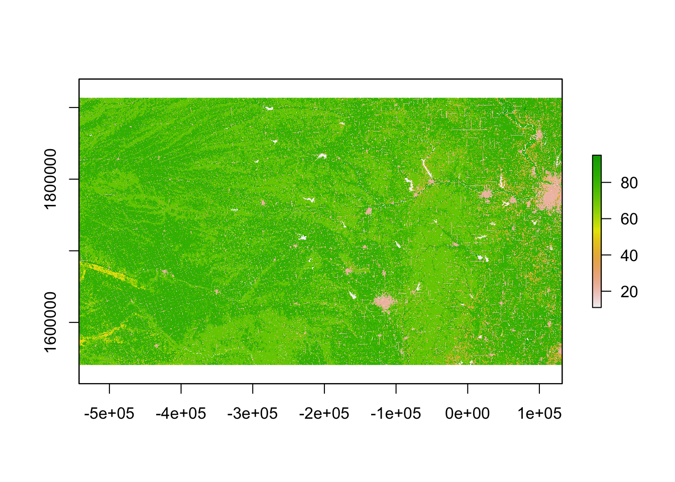
- Transformations and coordinate reference systems
- Not all spatial files have the same coordinate reference systems.
library(sp)

sf.kansas <- spTransform(sf.kansas, crs(rl.nlcd2011))

plot(rl.nlcd2011)
plot(sf.kansas, add = TRUE, lwd = 4)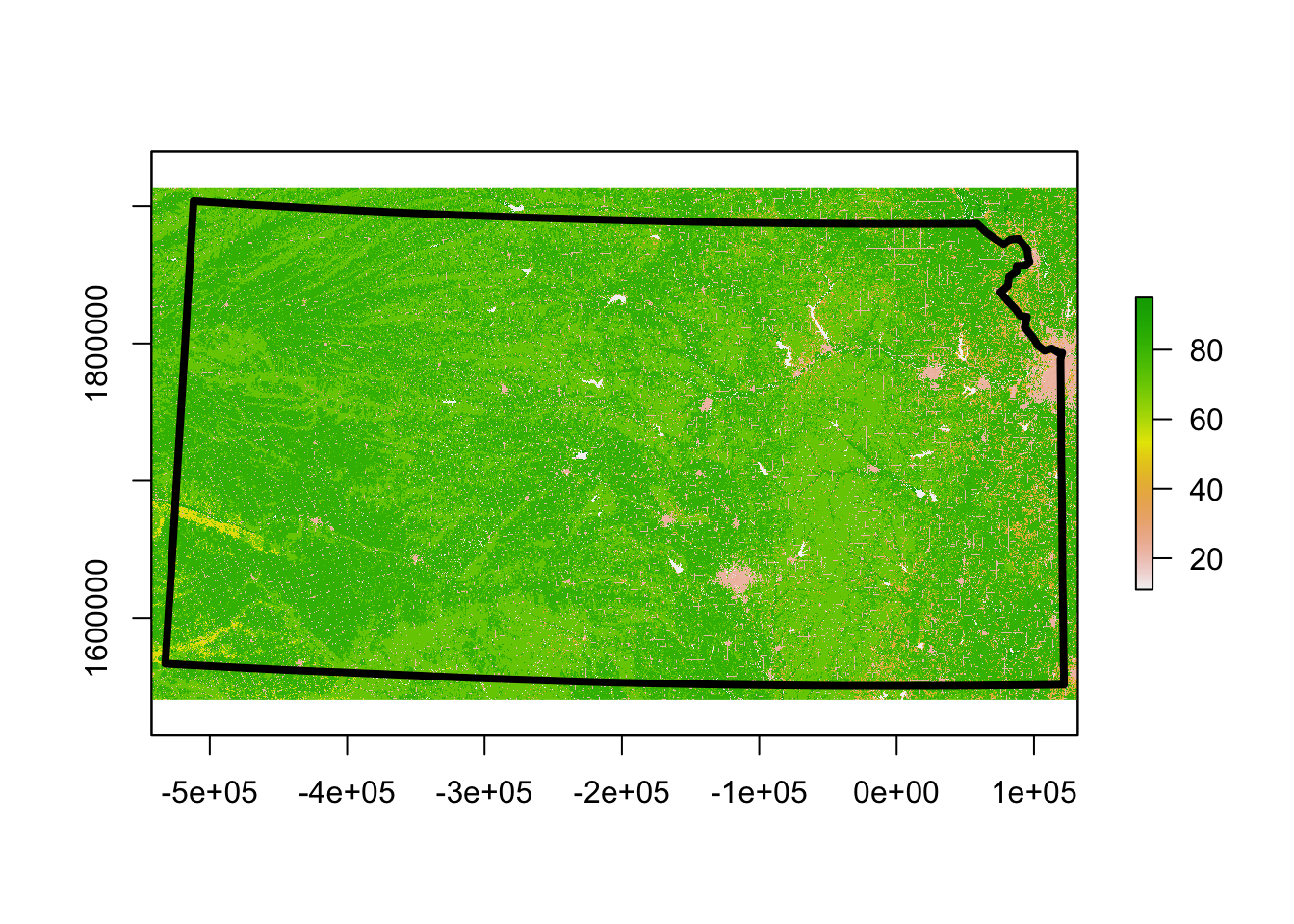
11.3.3 Points
- Point files are created from coordinates (and a corresponding coordinate system)
- Example: Plot location of Dickens Hall
pt.dickens <- data.frame(long = -96.579382, lat = 39.190433) #Location of Dickens Hall
coordinates(pt.dickens) = ~long + lat
proj4string(pt.dickens) <- CRS("+proj=longlat +datum=WGS84 +no_defs +ellps=WGS84 +towgs84=0,0,0")
pt.dickens <- spTransform(pt.dickens, crs(rl.nlcd2011))
plot(rl.nlcd2011)
plot(sf.kansas, add = TRUE, lwd = 4)
plot(pt.dickens, add = TRUE, col = "gold", pch = 20, cex = 3)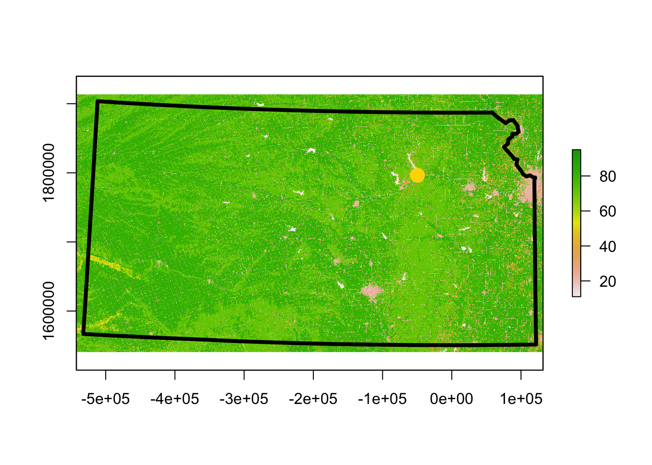 - Get the landcover type at this location
extract(rl.nlcd2011, pt.dickens) # See legend at https://www.mrlc.gov/data/legends/national-land-cover-database-2011-nlcd2011-legend##
## 2311.3.4 Summary
- There are entire courses on what we covered today
- Example (GIS certificate at KSU)
- This is an area that is rapidly developing
- New R packages to automate data downloads
- New sources of data (e.g., UAS)
- Best and most up-to-date resources are usually found be doing a Google search
- Learning how to use R as a GIS can take some time and be frustrating at first