6 Day 6 (February 5)

6.1 Announcements

Office hours on Friday 3pm Dickens Hall 109.
The first part of Activity 2 is posted
Read and re-read pgs. 10-14 of Spatio-temporal statistics with R.
Questions/clarifications from journals
- “I’m just an amateur with R and I’m trying to learn the language to become as good as you’re; just though to ask if there’s any R learning book you would recommend?”
- “For the class project, I’m just wondering if someone had a dataset say like rainfall (hourly) and then, they want to evaluate machine learning models which can accurately predict the rainfall, would such a topic be considered as a spatial-temporal one (since it has the time aspect?) would it help someone uncover and learn the course’s principles?”
- “One thing I’m struggling to understand is how distributions affect linear regression. It’s becoming clearer to me that while almost everything I’ve learned up until this point has been based on normal distribution, a lot of data is in fact… not normal.”
- “When is it justified to change our assumption about the error distribution? Especially in the absence of biologically reasonable explanations.”
- “Something that I am struggling to understand from within the past 24 hours is how to implement the constraint that a single β is non-negative in the cars example.”

6.2 Distribution theory review

Moments of a distribution
Revisiting the cars example[(Download example here)]
A few other examples where moments matter.
- Link to paper

6.3 Mathematical model review

Mathematical models are deterministic equations that describe the relationship between input variables and an output variable
Common types of mathematical models used for spatio-temporal statistics
- Linear equations
  - Scalar form: \(\mu=\beta_{0}+\beta_{1}x_{1}+\beta_{2}x_{2}+\ldots+\beta_{p}x_{p}\)
  - Vector form: \(\boldsymbol{\mu}=\beta_{0}+\beta_{1}\mathbf{x}_{1}+\beta_{2}\mathbf{x}_{2}+\ldots+\beta_{p}\mathbf{x}_{p}\)
  - Matrix form: \(\boldsymbol{\mu}=\mathbf{X}\boldsymbol{\beta}\)
- Non-linear equations Scalar form: \(\mu = e^{\beta_{0}+\beta_{1}x_{1}+\beta_{2}x_{2}+\ldots+\beta_{p}x_{p}}\)
- Difference equations
  - Scalar form: \(\mu_{t+1} = \phi\mu_{t}\)
- Differential equations
  - Scalar form: \(\frac{d\mu(t)}{dt}=\gamma\mu(t)\)

6.4 Summary of statistical models

Probability distributions and mathematical models are the building block for most (parametric) statistical models
- Agent-based models simulation models are also widely used but rarely using statistical approaches (Epstein and Axtell 1996; Heard et al. 2015)

6.4.1 Motivating data example

Whooping cranes

Data set

url <- "https://www.dropbox.com/scl/fi/kxzc8fmomkigcrxyjjmdp/Butler-et-al.-Table-1.csv?rlkey=61ey3q1jc4rsor257uy4080j3&dl=1"
df1 <- read.csv(url)

plot(df1$Winter, df1$N, xlab = "Year", ylab = "Population count (z)", xlim = c(1940,
    2020), ylim = c(0, 300), typ = "b", cex = 0.8, pch = 20, col = rgb(0.7, 0.7,
    0.7, 0.9))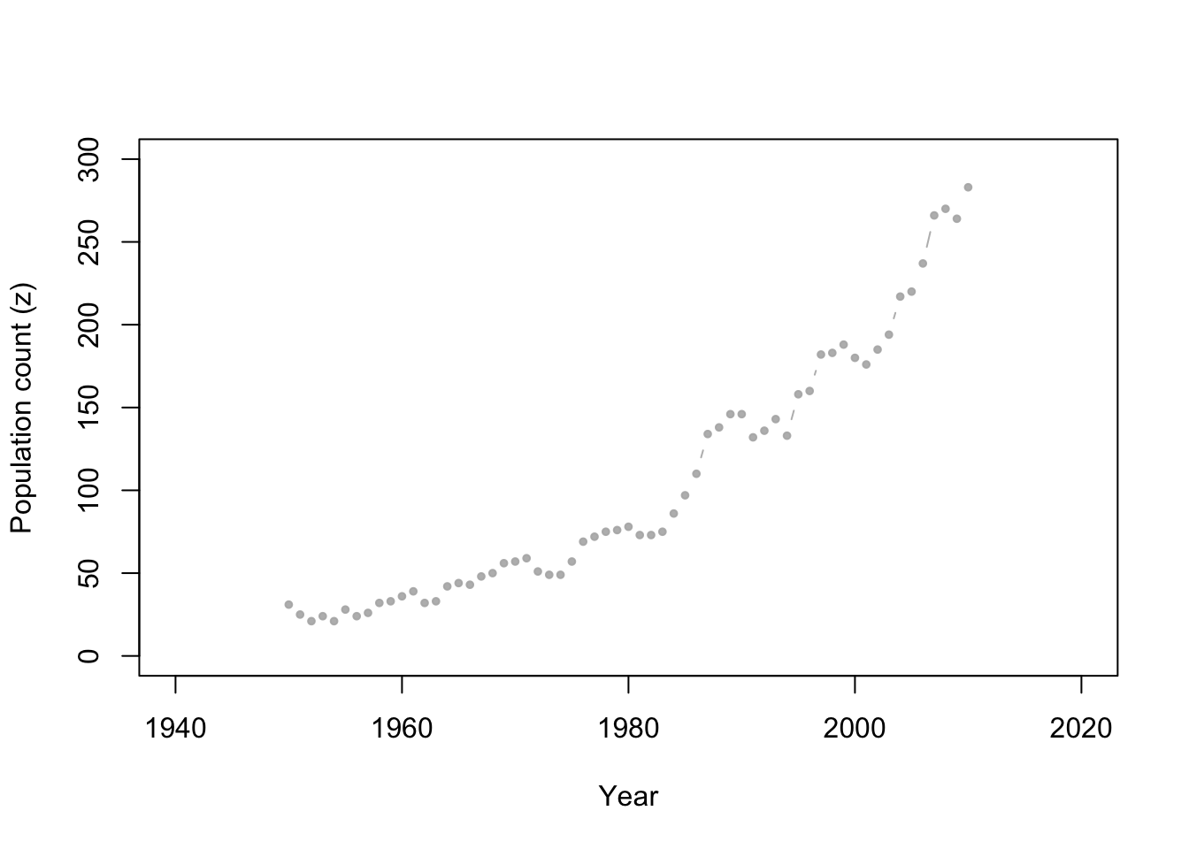

Live example Download R code here
We want to build a statistical model that enables
- Predictions and forecasts of the true population size
- Statistical inference on the date when the population will be larger than 1000 individuals

\[[\mathbf{z}_{\text{pred}}|\mathbf{z}]=\int\int\mathbf{[z}_{\text{pred}}|\mathbf{y},\boldsymbol{\theta}][\mathbf{y}|\boldsymbol{\theta}][\boldsymbol{\theta}|\mathbf{z}]d\mathbf{y}d\mathbf{\boldsymbol{\theta}}\]
- White board whooping crane example of BHM.