12 Day 12 (February 26)

12.1 Announcements

• Activity 3 is posted

• Final project proposals (if you have a 10/10 grade on Canvas start working!)

• Office hours have been moved to 2-3pm today (Dickens Hall 109)

• Read Ch. 4 pgs 137-192

  • Concepts and Synthesis paper

• Questions/clarifications from journals

  • Use of other software for class project (e.g., python, matlab, SAS, etc)
  • Trevor is getting old and python may be a better option for this class.
  • If you drop the NAs but keep the zeros, what missingness assumption are you making? (see monograph here)
  • “I’m still struggling to understand how we decide which probability distribution is appropriate for a given problem. For example, in the rainfall example we used a normal distribution even though rainfall can’t be negative, and that confused me because the normal distribution allows both negative and positive values.”

12.2 Extreme precipitation in Kansas

• Note, this is essentially the same as activity 2

• On September 3, 2018 there was an extreme precipitation event that resulted in flooding in Manhattan, KS and the surrounding areas. If you would like to know more about this, check out this link and this video here and here.

• My process

  • Determine the goals of the study
  • Data acquisition
    • Live demonstration (Download R code here)
  • Exploratory data analysis
    • Live demonstration
  • The model building process
    • 1). Choose appropriate PDFs or PMFs for the data, process, and parameter models
    • 2). Choose appropriate mathematical models for the “parameters” or moments of the PDFs/PMFs from step 1.
      
    • 3). Choose an algorithm fit the statistical model to the data
    • 4). Make statistical inference (e.g., calculate derived quantities and summarize the posterior distribution)
  • Model checking, improvements, validation, and selection (Ch. 6)

• What we will need to learn

  • How to use R as a geographic information system
  • New general tools from statistics
    • Gaussian process
    • Metropolis and Metropolis–Hastings algorithms
    • Gibbs sampler
  • How to use the hierarchical modeling framework to describe Kriging
    • Hierarchical Bayesian model vs. “empirical” hierarchical model
  • Specialized language used in spatial statistics (e.g., range, nugget, variogram)

12.2.1 Multivariate normal distribution

• Multivariate normal distribution

• \(\boldsymbol{\eta}\sim\text{N}(\mathbf{0},\sigma^{2}\mathbf{R})\)

  • Definitions

• Correlation matrix – A positive semi-definite matrix whose elements are the correlation between observations

• Correlation function – A function that describes the correlation between observations

• Example correlation matrices

• Compound symmetry \[\mathbf{R}=\left[\begin{array}{cccccc} 1 & 1 & 0 & 0 & 0 & 0\\ 1 & 1 & 0 & 0 & 0 & 0\\ 0 & 0 & 1 & 1 & 0 & 0\\ 0 & 0 & 1 & 1 & 0 & 0\\ 0 & 0 & 0 & 0 & 1 & 1\\ 0 & 0 & 0 & 0 & 1 & 1 \end{array}\right]\]

  • AR(1) \[\mathbf{R(\phi})=\left[\begin{array}{ccccc} 1 & \phi^{1} & \phi^{2} & \cdots & \phi^{n-1}\\ \phi^{1} & 1 & \phi^{1} & \cdots & \phi^{n-2}\\ \phi^{2} & \phi^{1} & 1 & \vdots & \phi^{n-3}\\ \vdots & \vdots & \vdots & \ddots & \ddots\\ \phi^{n-1} & \phi^{n-2} & \phi^{n-3} & \ddots & 1 \end{array}\right]\:\]

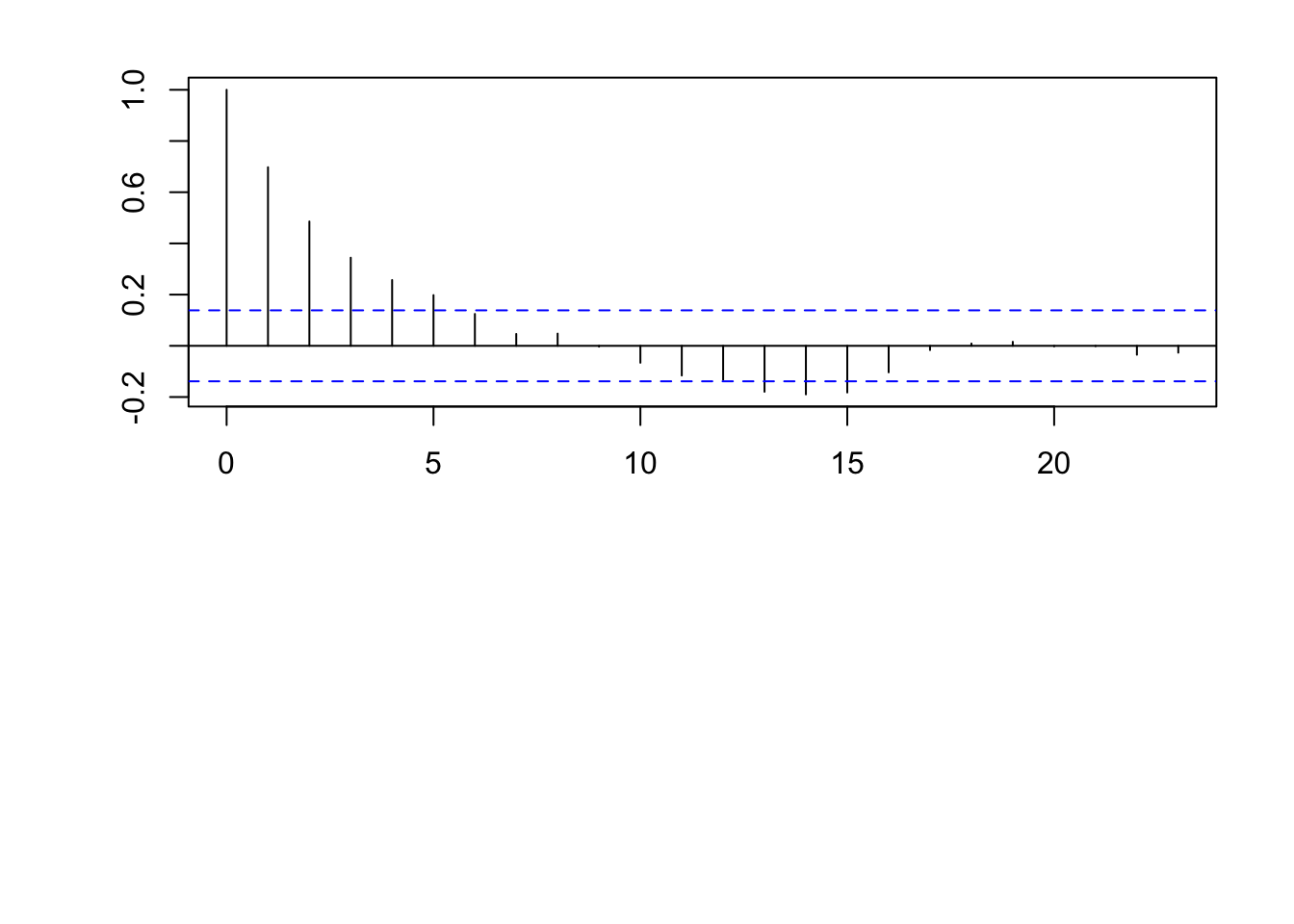
    • Example simulating from \(\boldsymbol{\eta}\sim\text{N}(\mathbf{0},\sigma^{2}\mathbf{R})\) in R

    n <- 200
    x <- 1:n
    I <- diag(1, n)
    sigma2 <- 1
    
    library(MASS)
    set.seed(2034)
    eta <- mvrnorm(1, rep(0, n), sigma2 * I)
    cor(eta[1:(n - 1)], eta[2:n])

    ## [1] -0.06408623

    acf(eta)

    

    par(mfrow = c(2, 1))
    par(mar = c(0, 2, 0, 0), oma = c(5.1, 3.1, 2.1, 2.1))
    plot(x, eta, typ = "l", xlab = "", xaxt = "n")
    abline(a = 0, b = 0)
    
    n <- 200
    x <- 1:n  # Must be equally spaced
    phi <- 0.7
    R <- phi^abs(outer(x, x, "-"))
    sigma2 <- 1
    set.seed(1330)
    eta <- mvrnorm(1, rep(0, n), sigma2 * R)
    cor(eta[1:(n - 1)], eta[2:n])

    ## [1] 0.7015304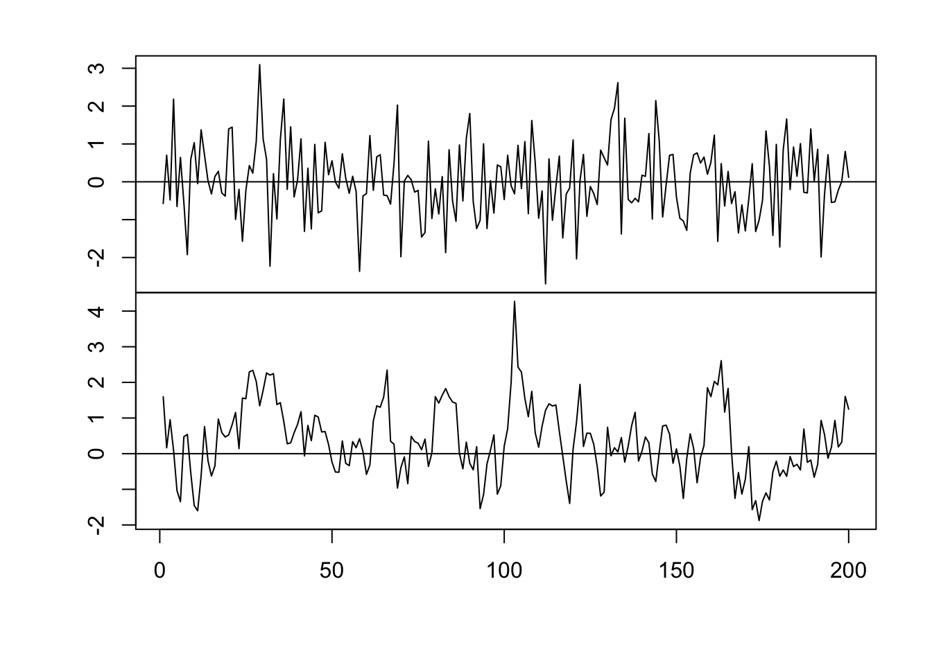

    plot(x, eta, typ = "l")
    abline(a = 0, b = 0)

    

    acf(eta)

    

  • Example correlation functions

  • Gaussian correlation function \[r_{ij}(\phi)=e^{-\frac{d_{ij}^{2}}{\phi}}\] where \(d_{ij}\) is the “distance” between locations i and j (note that \(d_{ij}=0\) for \(i=j\)) and \(r_{ij}(\phi)\) is the element in the \(i^{\textrm{th}}\) row and \(j^{\textrm{th}}\) column of \(\mathbf{R}(\phi)\).

    library(fields)
    n <- 200
    x <- 1:n
    phi <- 40
    d <- rdist(x)
    R <- exp(-d^2/phi)
    sigma2 <- 1
    
    set.seed(4673)
    eta <- mvrnorm(1, rep(0, n), sigma2 * R)
    plot(x, eta, typ = "l")
    abline(a = 0, b = 0)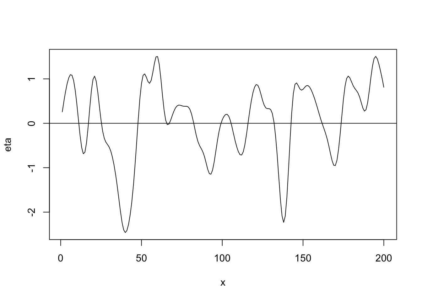

    

    cor(eta[1:(n - 1)], eta[2:n])

    ## [1] 0.9718077

• Linear correlation function \[r_{ij}(\phi)=\begin{cases} 1-\frac{d_{ij}}{\phi} &\text{if}\ d_{ij}<0\\ 0 &\text{if}\ d_{ij}>0 \end{cases}\]

  library(fields)
  n <- 200
  x <- 1:n
  phi <- 40
  d <- rdist(x)
  R <- ifelse(d < phi, 1 - d/phi, 0)
  sigma2 <- 1
  
  set.seed(4803)
  eta <- mvrnorm(1, rep(0, n), sigma2 * R)
  plot(x, eta, typ = "l")
  abline(a = 0, b = 0)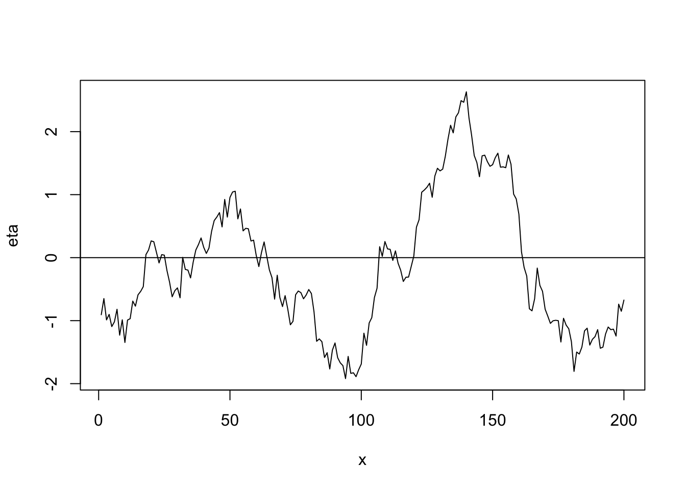

  

  cor(eta[1:(n - 1)], eta[2:n])

  ## [1] 0.9774775

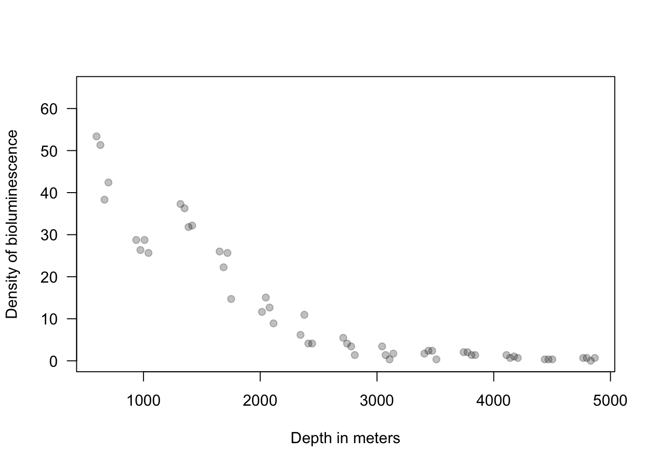
12.3 Linear models for correlated errors

• Motivating example

  ISIT <- read.table("https://www.dropbox.com/scl/fi/n5ku9crpsr384p9z2rc8b/bioluminescence.txt?rlkey=airzs2ukql4g0hqxjr72re53j&dl=1",
      header = TRUE)
  
  Sources16 <- ISIT$Sources[ISIT$Station == 16]
  Depth16 <- ISIT$SampleDepth[ISIT$Station == 16]
  Sources16 <- Sources16[order(Depth16)]
  Depth16 <- sort(Depth16)
  plot(Depth16, Sources16, las = 1, ylim = c(0, 65), col = rgb(0, 0, 0, 0.25), pch = 19,
      ylab = "Density of bioluminescence", xlab = "Depth in meters")