5 Day 5 (February 3)

5.1 Announcements

• Activity 1.

  • “What did you do?”
  • Comment about giving me just R code
  • Comment about ggplot and prediction intervals
  • Comment about automation, AI, etc.

• The first part of Activity 2 is posted

• Read and re-read pgs. 10-14 of Spatio-temporal statistics with R.

• Questions/clarifications from journals

  • A lot of this is covered in 6.3 and 6.4 of the book (pgs. 268-284)
  • “In class today, I learned that predictive accuracy in time series forecasting is not just about getting a close point estimate, but also about whether the forecast distribution is reasonable.”
  • “Following up on the cross-validation discussion, I didn’t fully understand why a model would be considered good when, during calibration, 95% of the estimated data points fall within the prediction interval (PI).”
  • “Something that I am struggling to understand from within the past 24 hours is what kind of spatio-temporal methods are we supposed to try on the final project? Are we supposed to choose a method from the textbook ourselves or are we going to discuss some common methods in class?”
  • “Can we assume that the model with the lowest AICc would have the best predictive accuracy?” (See Gelman paper for quote)
  • “I think I’m a little confused about the difference between calibration and cross validation.”
  • Trevor’s thoughts about cross validation and information-based criteria for model selection/evaluation of predictive performance

5.2 Distribution theory review

• Probability density functions (PDF) and probability mass functions (PMF)

  • Normal distribution (continuous support)
  • Binomial distribution (discrete support)
  • Poisson distribution (discrete support)
  • And many more

• Distributions in R

  • PDF of the normal distribution \[[z|\mu,\sigma^2] = \frac{1}{\sqrt{2\pi\sigma^2}}\textit{e}^{-\frac{1}{2\sigma^2}(z - \mu)^2}\]
    • \(z\) is the random variable
    • \(\mu\) and \(\sigma^2\) are the parameters
  • PDFs & PMFs in R
    • ?dnorm
  • Generate random variables (\(z\)) from a PDF (e.g., \(z_i\sim\text{N}(\mu,\sigma^2)\))

  z <- rnorm(n = 5, mean = 0, sd = 1)
  z    

  ## [1] -0.1559493 -1.6306246  0.7765410  0.1257194  0.5299815

  • Histogram representation of a PDF

  library(latex2exp)
  z <- rnorm(n = 10000, mean = 0, sd = 1)
  hist(z,freq=FALSE,col="grey",main = "",
    xlab= TeX('$\\textit{z}$'),
    ylab = TeX('$\\lbrack\\textit{z}|\\mu,\\sigma^2\\rbrack$'))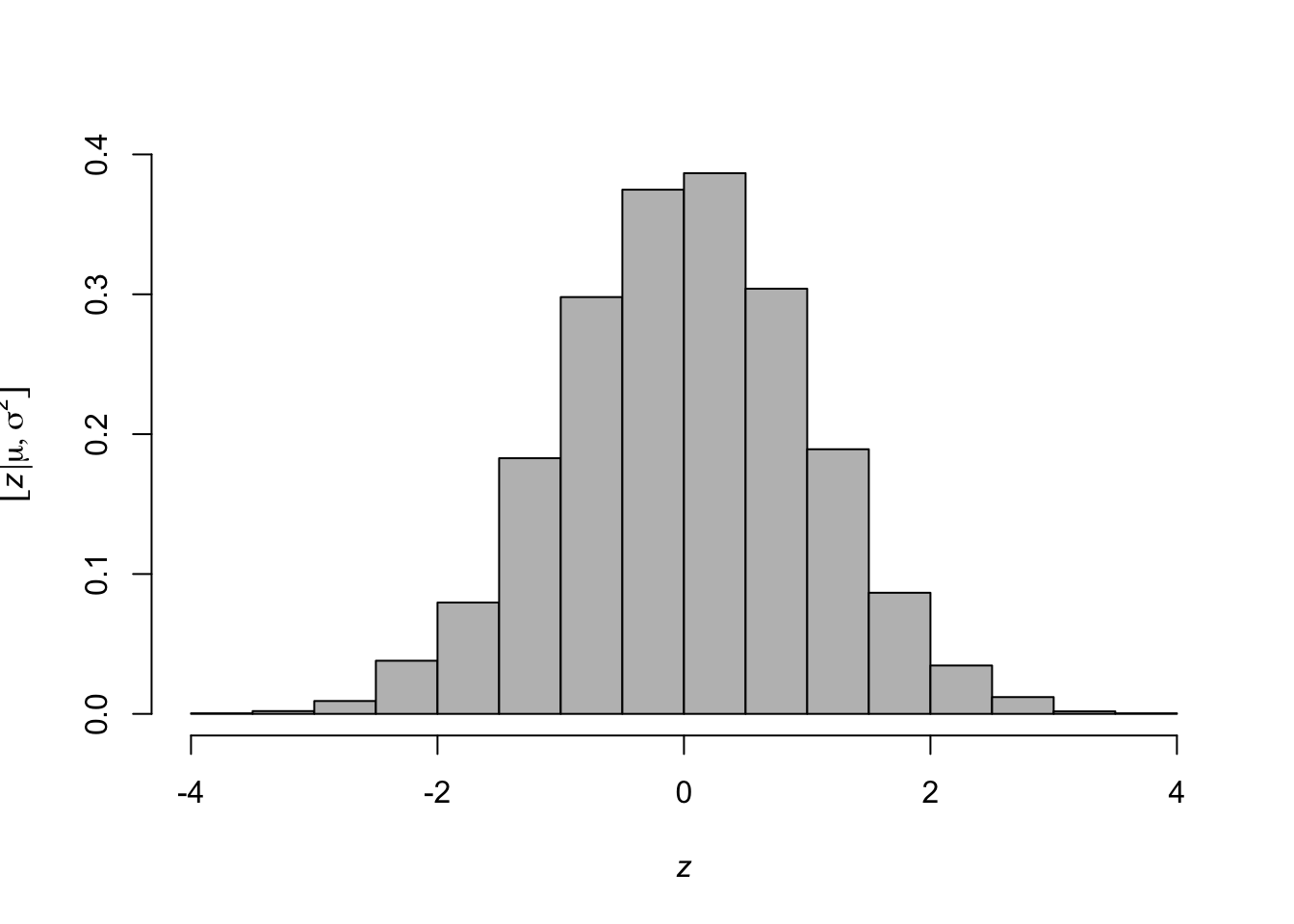

  

  • Plot a PDF in R

  curve(expr = dnorm(x = x, mean = 0, sd = 1), from = -10, to = 10,
    xlab= TeX('$\\textit{z}$'),
    ylab = TeX('$\\lbrack\\textit{z}|\\mu,\\sigma^2\\rbrack$'))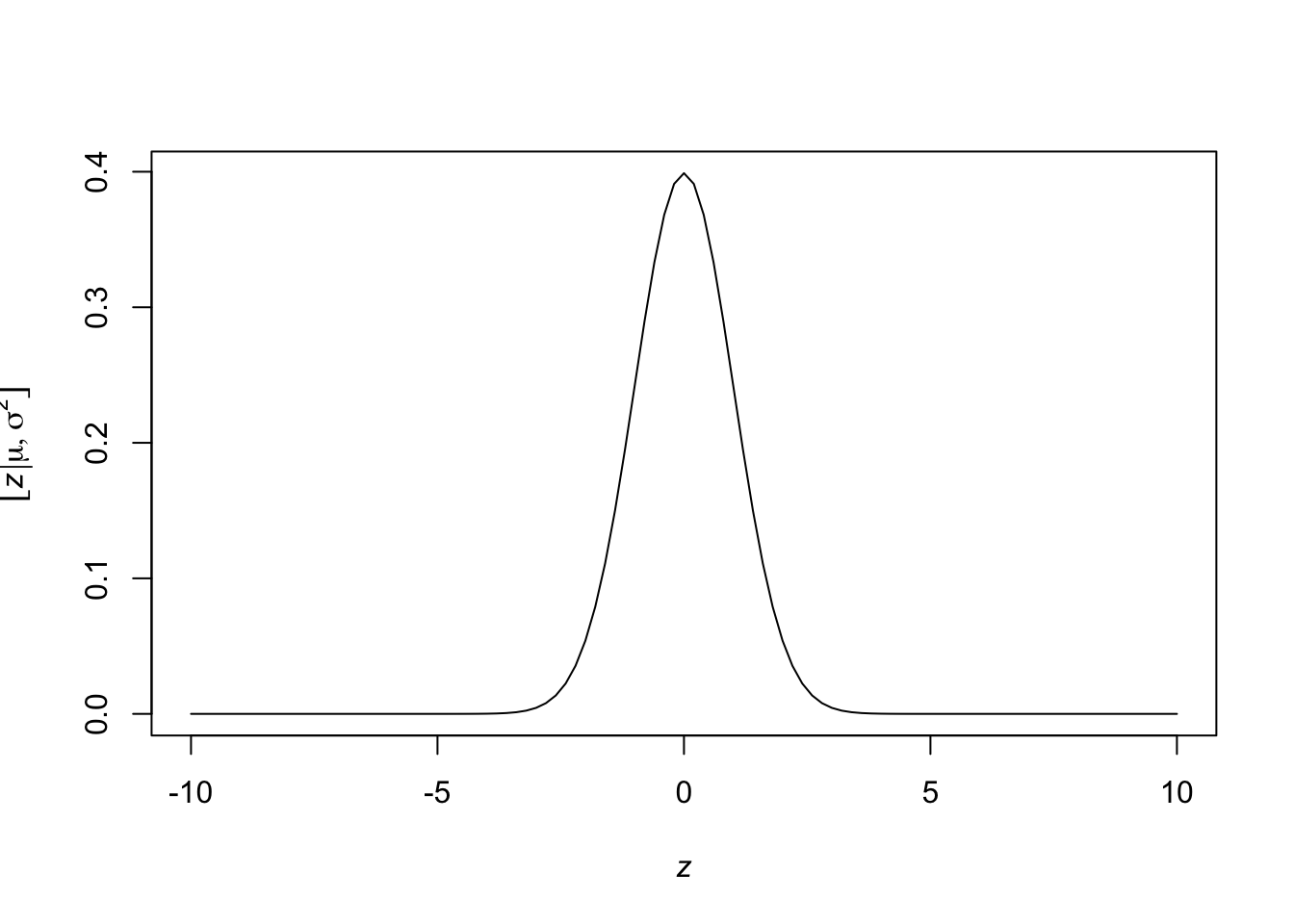

  

  • Evaluate the “likelihood” at a given value of the parameters

  dnorm(x = 1.759, mean = 0, sd = 1, log = FALSE)

  ## [1] 0.08492566

  • Other distributions

  rpois(n = 5, lambda = 2)
  rbinom(n = 5, size = 10, prob = 0.5)    
  runif(n = 5,min = 0,max = 3)
  rt(n = 5,df = 1)
  rcauchy(n = 5, location = 2, scale = 4)

  • See stats package for more information
    

• Making your own functions for a distribution

  • PDF of the exponential distribution \[[z|\lambda] = \lambda\textit{e}^{-\lambda z}\]
  • Make your own function for the PDF of the exponential distribution

  dexp <- function(z, lambda){lambda*exp(-lambda*z)}

  • Make your own function to simulate random variables from the exponential distribution using the inverse probability integral transform

  rexp <- function(n, lambda){
    u <- runif(n)
    -1/lambda*log(1-u)
  }

  • Make histogram by sampling from rexp() and overlay the PDF using dexp()

  z <- rexp(n = 10000, lambda = 1)
  hist(z,freq=FALSE,col="grey",main = "",
    xlab= TeX('$\\textit{z}$'),
    ylab = TeX('$\\lbrack\\textit{z}|\\lambda\\rbrack$'))
  curve(expr = dexp(z = x,lambda = 1), from = 0, to = 10, 
    add = TRUE,col = "deepskyblue",lwd = 3)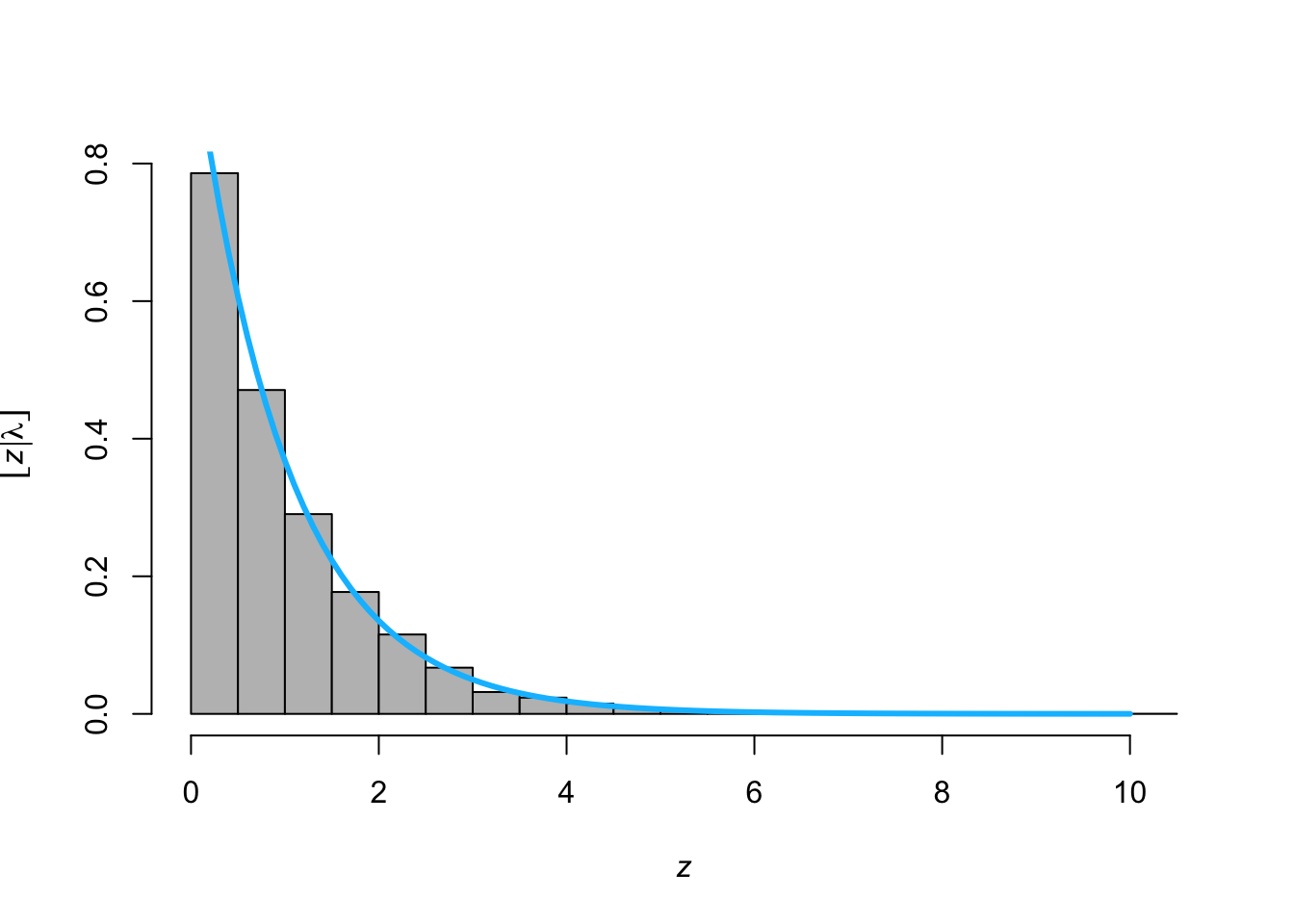

  

• Moments of a distribution

  • First moment: \(\text{E}(z) = \int z [z|\theta]dz\)
  • Second central moment: \(\text{Var}(z) = \int (z -\text{E}(z))^2[z|\theta]dz\)
  • Note that \([z|\theta]\) is an arbitrary PDF or PMF with parameters \(\theta\)
  • Example normal distribution \[\begin{eqnarray} \text{E}(z) &=& \int_{-\infty}^\infty z\frac{1}{\sqrt{2\pi\sigma^2}}\textit{e}^{-\frac{1}{2\sigma^2}(z - \mu)^2}dz\\&=& \mu \end{eqnarray}\] \[\begin{eqnarray} \text{Var}(z) &=& \int_{-\infty}^\infty (z-\mu)^2\frac{1}{\sqrt{2\pi\sigma^2}}\textit{e}^{-\frac{1}{2\sigma^2}(z - \mu)^2}dz\\&=& \sigma^2 \end{eqnarray}\]
  • Example exponential distribution\[\begin{eqnarray} \text{E}(z) &=& \int_{0}^\infty z\lambda\textit{e}^{-\lambda z}dz\\&=& \frac{1}{\lambda} \end{eqnarray}\]\[\begin{eqnarray}\text{Var}(z) &=& \int_{0}^\infty (z-\mu)^2\lambda\textit{e}^{-\lambda z}dz\\&=& \frac{1}{\lambda^2} \end{eqnarray}\]

• Revisiting the cars example[(Download example here)]