26 Day 26 (April 23)
26.1 Announcements
- Stats seminar today
- Calendar
- Workday on Tuesday 4/28.
- Lecture on Tuesday 4/30
- Lecture on Tuesday 5/5
- Lecture on Tuesday 5/7
- Next week and the week after is very open if you need to meet.
- Presentation dates/time? My preference for presentations is May 4-8. Please send me an email (thefley@ksu.edu) and provide three 30 min long times/dates that work for you.
- Questions about the peer review?
- You need to find a person/group to exchange your material with.
- If you can’t find a person/group, I can play matchmaker!
- Read this paper (link)
- Toy example demonstrating ideas from the paper (link)
- Questions/clarifications from journals
- “Do you think it would be interesting to add a decay distance function to the earthquake model? Whenever I have “distance to [something]” as a response variable I feel like I always want to go for decay distance instead, because it usually makes more sense in the wildlife world biologically”
- “Regarding regression dilution, you mentioned that if we see an effect still when the dilution is present, we can probably assume that the effect is stronger than what we’re actually seeing. Are there cases where this might not be true?” Yes! See here, here and here.
- “If I understood correctly, you were comfortable ignoring measurement error in latitude and longitude, assuming locations are accurate. But would you make the same assumption for the number of observations over time? What I’m struggling with is how to account for possible measurement or observation error over time, since it seems unrealistic to assume the data are fully comparable across years. The increase could be due to changes in monitoring, detection thresholds, or reporting, not only a real increase in earthquakes.”
- “I realized today that the use of different distributions is something we have focused on a lot since the beginning of the class, and I paid a lot of attention to it at that time. However, today I noticed that I have been doing analyses in other projects again without even thinking about which distributions might be better, just using Normal.”
- “Then, to check whether I am understanding the main idea, is the IPP distribution used to describe the location of a random number of events within a geographic region, where that spatial distribution is explained by an intensity function? Is that intensity function similar to controlling the expected number of events over space?”
26.2 Earthquake data
-
library(sf)
library(sp)
library(raster)
library(lubridate)
library(animation)
library(gifski)


# Download shapefile of Kansas from census.gov
download.file("http://www2.census.gov/geo/tiger/GENZ2015/shp/cb_2015_us_state_20m.zip",
    destfile = "states.zip")
unzip("states.zip")
sf.us <- st_read("cb_2015_us_state_20m.shp", quiet = TRUE)
sf.kansas <- sf.us[48, 6]
sf.kansas <- as(sf.kansas, "Spatial")

# Load earthquake data
url <- "https://www.dropbox.com/scl/fi/uhicc7qo4zcxeq79y1eh9/ks_earthquake_data.csv?rlkey=lbq8kxzx9g067domp46ffh7jw&dl=1"
df.eq <- read.csv(url)
df.eq$Date.time <- ymd_hms(df.eq$Date.time)
pts.eq <- SpatialPointsDataFrame(coords = df.eq[, c(3, 2)], data = df.eq[, c(1, 4)],
    proj4string = crs(sf.kansas))

# Plot spatial map earthquake data
par(mar = c(5.1, 4.1, 4.1, 8.1), xpd = TRUE)
plot(sf.kansas, main = "")
points(pts.eq, col = rgb(0.4, 0.8, 0.5, 0.3), pch = 21, cex = pts.eq$Magnitude/3)
legend("right", inset = c(-0.25, 0), legend = c(1, 2, 3, 4, 5), bty = "n", text.col = "black",
    pch = 21, cex = 1.3, pt.cex = c(1, 2, 3, 4, 5)/3, col = rgb(0.4, 0.8, 0.5, 0.6))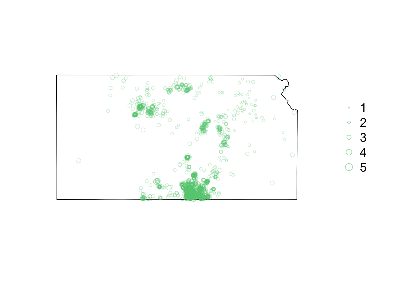
# Plot timeseries of earthquake data
plot(as.numeric(names(table(year(df.eq$Date.time)))), c(table(year(df.eq$Date.time))),
    xlab = "Year", ylab = "Number of Earthquakes in KS", pch = 20)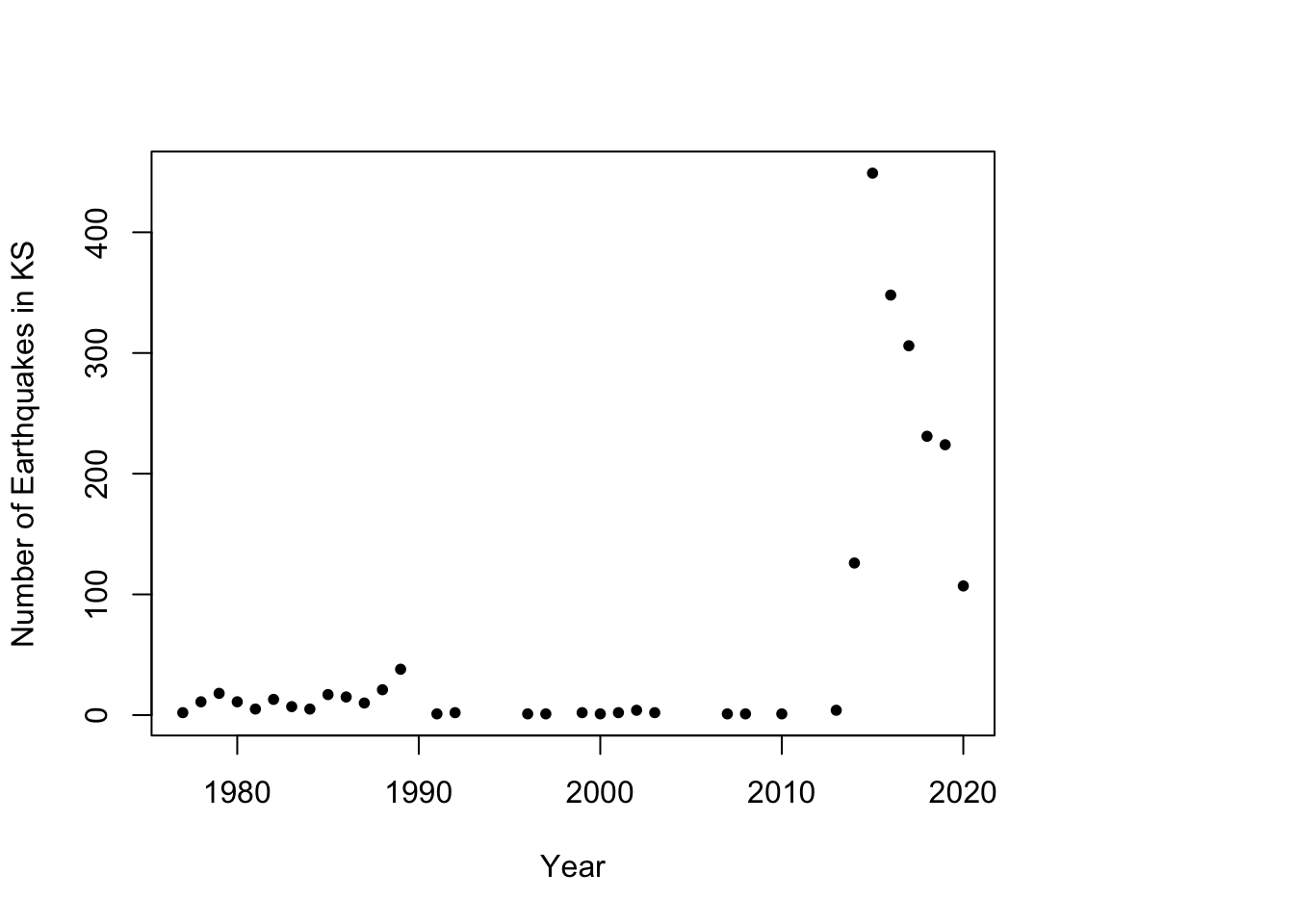
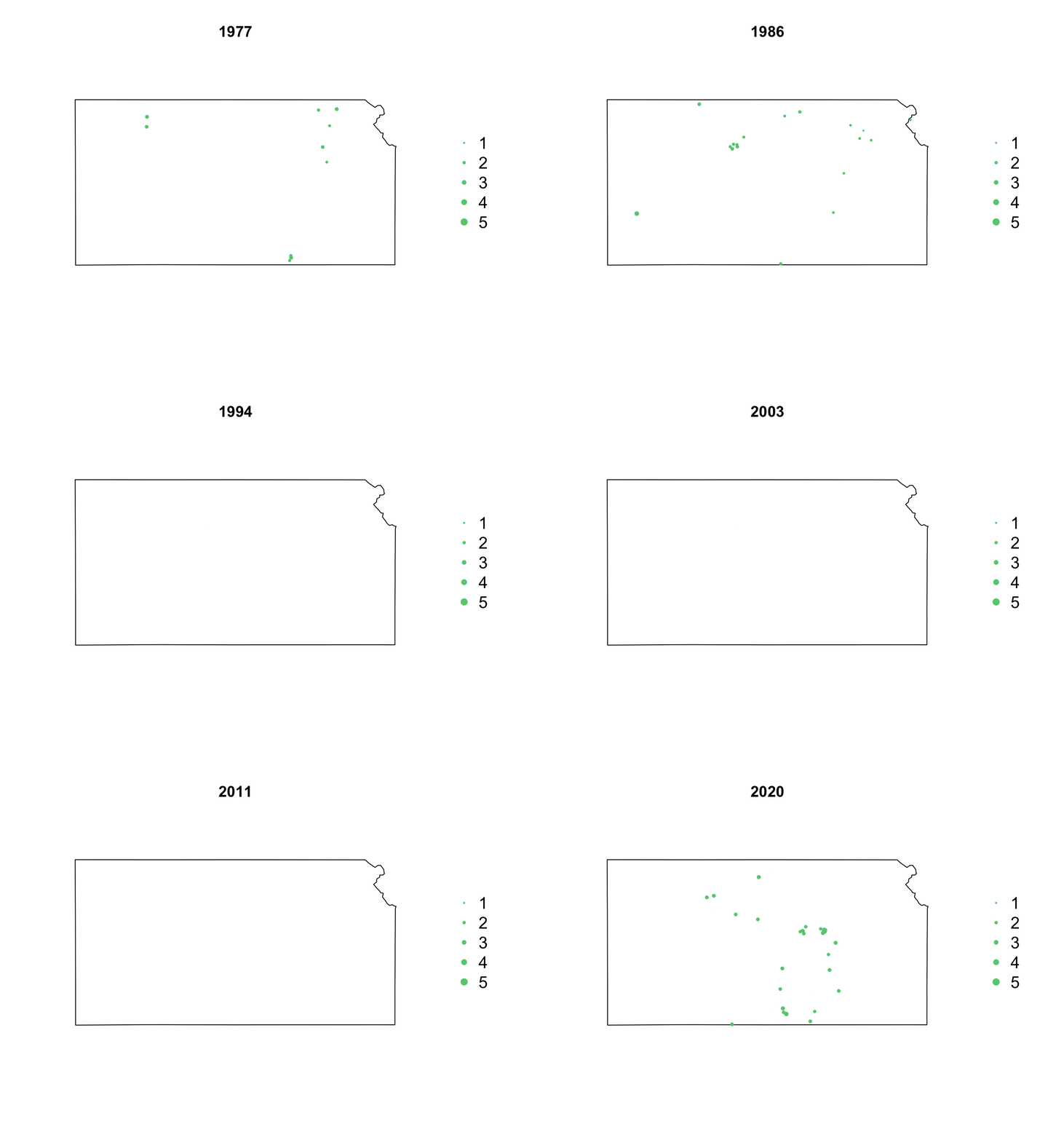
- Animation of Kansas Earthquake data
# Make animation of earthquake data
date <- seq(as.Date("1977-1-1"), as.Date("2020-10-31"), by = "year")
t <- round(time_length(interval(min(date), pts.eq$Date.time), "year"))

for (i in 1:length(date)) {
    par(mar = c(5.1, 4.1, 4.1, 8.1), xpd = TRUE)
    plot(sf.kansas, main = year(date[i]))
    legend("right", inset = c(-0.25, 0), legend = c(1, 2, 3, 4, 5), bty = "n", text.col = "black",
        pch = 20, cex = 1.3, pt.cex = c(1, 2, 3, 4, 5)/3, col = rgb(0.4, 0.8, 0.5,
            1))
    if (length(which(t == i)) > 0) {
        points(pts.eq[which(t == i), ], col = rgb(0.4, 0.8, 0.5, 1), pch = 20, cex = pts.eq[which(t ==
            i), ]$Magnitude/3)
    }
}
26.3 Spatio-temporal models for earthquake data
- What are the goals of our study?
- Prediction
- Make point and areal level predictions
- Inference
- Understand the spatio-temporal covariates that may increase or decrease the risk of an earthquake
- Prediction
- What auxiliary data do we need?
- Kansas oil and gas well data
- Descriptive vs. dynamic approach
- Write out statistical model for earthquake data
- R code to follow along