23 Day 23 (April 14)
23.1 Announcements
Questions about the peer review?
- You need to find a person/group to exchange your material with.
- If you can’t find a person/group, I can play matchmaker!
Read this paper (link)
Thursday (4/16) will be a work day
Tuesday (4/21) will be a work day
Read this paper (link)
- Toy example demonstrating ideas from the paper (link)
Questions/clarifications from journals
- “For the class project report, are we supposed to hand in a manuscript like or a report, from my understanding the two might be different, for example, a report might require a table of contents, list of acronyms used etc. which might not be necessary in the manuscript, I could be wrong!”
- “How much of industry uses spatiotemporal techniques and are at the cutting edge”
- “I’m still trying to understand what additive models are.”
- “The major challenge during this part of the course has been the writing component, including the literature review, introduction, and discussion, particularly in terms of developing clear storytelling. I also found it difficult to maintain focus on the main message I want to communicate through my research, especially after multiple data analysis steps that felt somewhat overwhelming.”
23.2 Spatio-temporal models for disease data
- Wrap up today
- Need to finish BYDV disease data
- Quick comment about pooled testing
- Need to finish mapping (See my own personal tutorial below)
- Example
- Data from Enders et al (2018) which is available on Dryad Digital Repository
- Example of my own person “tutorial” link
- R code for todays example
23.3 Earthquake data
-
library(sf)
library(sp)
library(raster)
library(lubridate)
library(animation)
library(gifski)


# Download shapefile of Kansas from census.gov
download.file("http://www2.census.gov/geo/tiger/GENZ2015/shp/cb_2015_us_state_20m.zip",
    destfile = "states.zip")
unzip("states.zip")
sf.us <- st_read("cb_2015_us_state_20m.shp", quiet = TRUE)
sf.kansas <- sf.us[48, 6]
sf.kansas <- as(sf.kansas, "Spatial")

# Load earthquake data
url <- "https://www.dropbox.com/scl/fi/uhicc7qo4zcxeq79y1eh9/ks_earthquake_data.csv?rlkey=lbq8kxzx9g067domp46ffh7jw&dl=1"
df.eq <- read.csv(url)
df.eq$Date.time <- ymd_hms(df.eq$Date.time)
pts.eq <- SpatialPointsDataFrame(coords = df.eq[, c(3, 2)], data = df.eq[, c(1, 4)],
    proj4string = crs(sf.kansas))

# Plot spatial map earthquake data
par(mar = c(5.1, 4.1, 4.1, 8.1), xpd = TRUE)
plot(sf.kansas, main = "")
points(pts.eq, col = rgb(0.4, 0.8, 0.5, 0.3), pch = 21, cex = pts.eq$Magnitude/3)
legend("right", inset = c(-0.25, 0), legend = c(1, 2, 3, 4, 5), bty = "n", text.col = "black",
    pch = 21, cex = 1.3, pt.cex = c(1, 2, 3, 4, 5)/3, col = rgb(0.4, 0.8, 0.5, 0.6))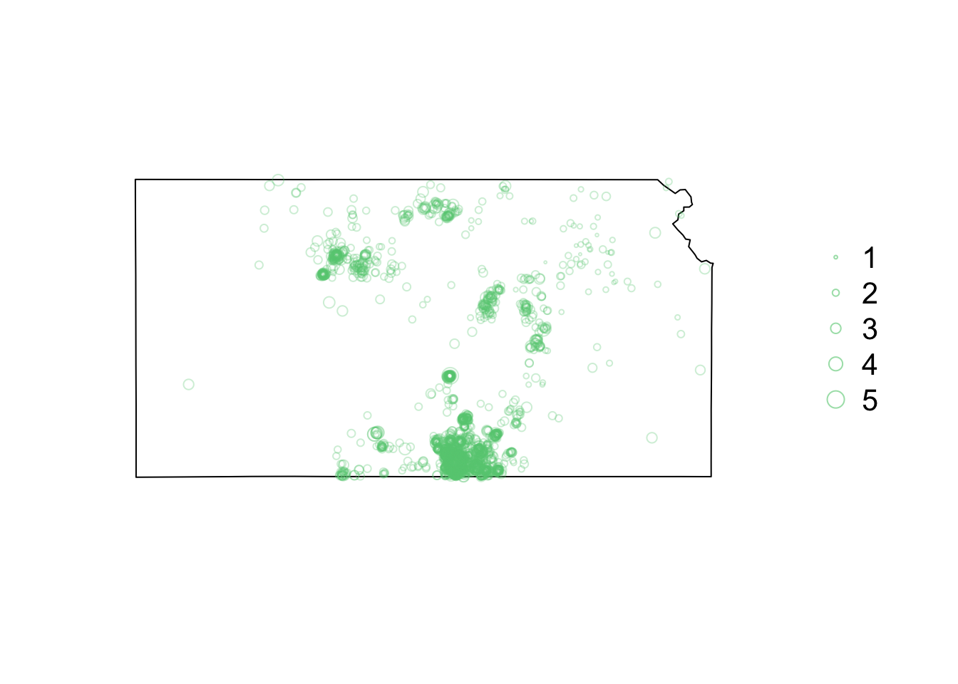
# Plot timeseries of earthquake data
plot(as.numeric(names(table(year(df.eq$Date.time)))), c(table(year(df.eq$Date.time))),
    xlab = "Year", ylab = "Number of Earthquakes in KS", pch = 20)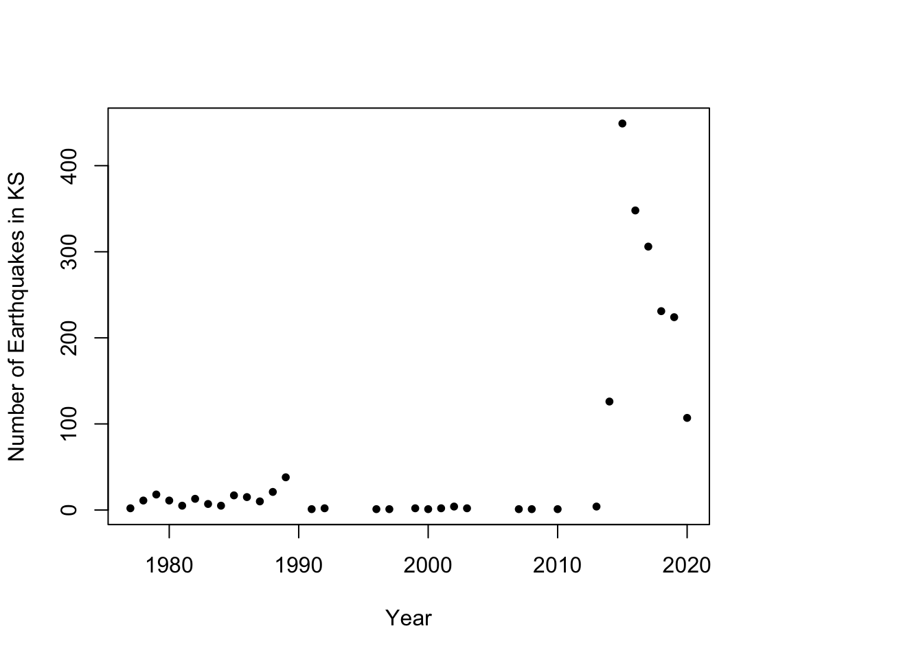
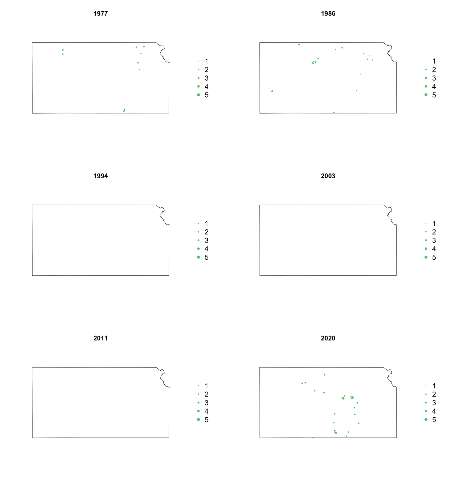
- Animation of Kansas Earthquake data
# Make animation of earthquake data
date <- seq(as.Date("1977-1-1"), as.Date("2020-10-31"), by = "year")
t <- round(time_length(interval(min(date), pts.eq$Date.time), "year"))

for (i in 1:length(date)) {
    par(mar = c(5.1, 4.1, 4.1, 8.1), xpd = TRUE)
    plot(sf.kansas, main = year(date[i]))
    legend("right", inset = c(-0.25, 0), legend = c(1, 2, 3, 4, 5), bty = "n", text.col = "black",
        pch = 20, cex = 1.3, pt.cex = c(1, 2, 3, 4, 5)/3, col = rgb(0.4, 0.8, 0.5,
            1))
    if (length(which(t == i)) > 0) {
        points(pts.eq[which(t == i), ], col = rgb(0.4, 0.8, 0.5, 1), pch = 20, cex = pts.eq[which(t ==
            i), ]$Magnitude/3)
    }
}
23.4 Spatio-temporal models for earthquake data
- What are the goals of our study?
- Prediction
- Make point and areal level predictions
- Inference
- Understand the spatio-temporal covariates that may increase or decrease the risk of an earthquake
- Prediction
- What auxiliary data do we need?
- Kansas oil and gas well data
- Descriptive vs. dynamic approach
- Write out statistical model for earthquake data
- R code to follow along