21 Day 21 (April 7)
21.1 Announcements
Read this paper (link)
Questions/clarifications from journals
- “A concern that I have is that I do not have the coordinates of the individual cores used to create each composite soil sample for phosphorus. The cores were taken at location within each plot, and the only average is the data we have.”
- “I am still struggling with how to balance simplicity and realism in a model. Sometimes using a simpler model seems more practical, especially when the dataset is limited, but I am not always sure when that simplification is reasonable and when it may remove important information.”
- “Since I am working on the project, I have a question around it. I’m having a hard time understanding why aggregating weather data by phenological stage isn’t showing any clear relationship with disease severity.”
21.2 Spatio-temporal models for disease data
Example
- Data from Enders et al (2018) which is available on Dryad Digital Repository
- Example of my own person “tutorial” link
- R code for todays example
library(sf)
library(sp)
library(raster)

url <- "https://www.dropbox.com/scl/fi/9ymxt900s77uq50ca6dgc/Enders-et-al.-2018-data.csv?rlkey=0rxjwleenhgu0gvzow5p0x9xf&dl=1"
df1 <- read.csv(url)
df1 <- df1[, c(1, 4, 5, 8, 9, 10)]  # Keep only the data on bird cherry-oat aphid

head(df1)
## BCOA BYDV.totalpos.BCOA BCOA.totaltested year long lat ## 1 12 2 10 2014 -95.16269 37.86238 ## 2 1 0 1 2014 -95.28463 38.29669 ## 3 2 0 2 2014 -95.33038 39.59482 ## 4 0 NA 0 2014 -95.32098 39.50696 ## 5 8 0 8 2014 -98.55469 38.48455 ## 6 1 0 1 2014 -98.84792 38.32772# Download shapefile of Kansas from census.gov download.file("http://www2.census.gov/geo/tiger/GENZ2015/shp/cb_2015_us_state_20m.zip", destfile = "states.zip") unzip("states.zip") sf.us <- st_read("cb_2015_us_state_20m.shp", quiet = TRUE) sf.kansas <- sf.us[48, 6] sf.kansas <- as(sf.kansas, "Spatial") # plot(sf.kansas,main='',col='white') # Make SpatialPoints data frame pts.sample <- data.frame(long = df1$long, lat = df1$lat, count = df1$BCOA, BYDV.pos = df1$BYDV.totalpos.BCOA, BYDV.tot = df1$BCOA.totaltested, BYDV.prop = df1$BYDV.totalpos.BCOA/df1$BCOA.totaltested) coordinates(pts.sample) = ~long + lat proj4string(pts.sample) <- CRS("+proj=longlat +datum=WGS84 +no_defs +ellps=WGS84 +towgs84=0,0,0") # Plot counts of Bird cherry-oat aphid par(mar = c(5.1, 4.1, 4.1, 8.1), xpd = TRUE) plot(sf.kansas, main = "Abundance of Bird Cherry-oat Aphid") points(pts.sample[, 1], col = rgb(0.4, 0.8, 0.5, 0.9), pch = ifelse(pts.sample$count > 0, 20, 4), cex = pts.sample$count/50 + 0.5) legend("right", inset = c(-0.25, 0), legend = c(0, 1, 10, 20, 40, 60), bty = "n", text.col = "black", pch = c(4, 20, 20, 20, 20, 20), cex = 1.3, pt.cex = c(0, 1, 10, 20, 40, 60)/50 + 0.5, col = rgb(0.4, 0.8, 0.5, 0.9))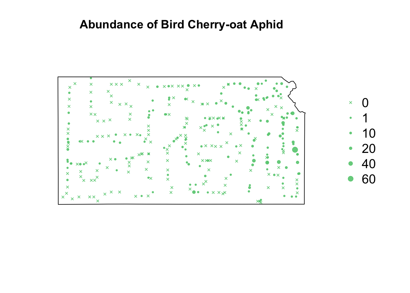
# Plot proportion of number of Bird cherry-oat aphid infected with BYDV
par(mar = c(5.1, 4.1, 4.1, 8.1), xpd = TRUE)
plot(sf.kansas, main = "Proportion infected")
points(pts.sample[, 4], col = rgb(0.8, 0.5, 0.4, 0.9), pch = ifelse(is.na(pts.sample$BYDV.prop) ==
    FALSE, 20, 4), cex = ifelse(is.na(pts.sample$BYDV.prop) == FALSE, pts.sample$BYDV.prop,
    0)/0.5 + 0.5)
legend("right", inset = c(-0.25, 0), legend = c("NA", 0, 0.25, 0.5, 0.75, 1), bty = "n",
    text.col = "black", pch = c(4, 20, 20, 20, 20, 20), cex = 1.3, pt.cex = c(0,
        0, 0.25, 0.5, 0.75, 1)/0.5 + 0.5, col = rgb(0.8, 0.5, 0.4, 0.9))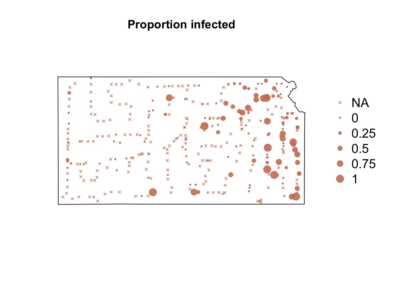
Study goals
- Make accurate predictions of vector abundance and probability of BYDV infection at times and locations where data was not collected.
- Understand the environmental factors (e.g., temperature) that influence the vector abundance and probability of BYDV infection.
Auxiliary data
- Weather/climate data
- Land cover data
- Crop data
Model choice: dynamic vs. descriptive spatio-temporal model?
- Class discussion
Next steps
- Write out the statistical model(s)
- Determine how we will evaluate how model(s)
- Determine how we will make inference
21.3 Earthquake data
-
library(sf)
library(sp)
library(raster)
library(lubridate)
library(animation)
library(gifski)


# Download shapefile of Kansas from census.gov
download.file("http://www2.census.gov/geo/tiger/GENZ2015/shp/cb_2015_us_state_20m.zip",
    destfile = "states.zip")
unzip("states.zip")
sf.us <- st_read("cb_2015_us_state_20m.shp", quiet = TRUE)
sf.kansas <- sf.us[48, 6]
sf.kansas <- as(sf.kansas, "Spatial")

# Load earthquake data
url <- "https://www.dropbox.com/scl/fi/uhicc7qo4zcxeq79y1eh9/ks_earthquake_data.csv?rlkey=lbq8kxzx9g067domp46ffh7jw&dl=1"
df.eq <- read.csv(url)
df.eq$Date.time <- ymd_hms(df.eq$Date.time)
pts.eq <- SpatialPointsDataFrame(coords = df.eq[, c(3, 2)], data = df.eq[, c(1, 4)],
    proj4string = crs(sf.kansas))

# Plot spatial map earthquake data
par(mar = c(5.1, 4.1, 4.1, 8.1), xpd = TRUE)
plot(sf.kansas, main = "")
points(pts.eq, col = rgb(0.4, 0.8, 0.5, 0.3), pch = 21, cex = pts.eq$Magnitude/3)
legend("right", inset = c(-0.25, 0), legend = c(1, 2, 3, 4, 5), bty = "n", text.col = "black",
    pch = 21, cex = 1.3, pt.cex = c(1, 2, 3, 4, 5)/3, col = rgb(0.4, 0.8, 0.5, 0.6))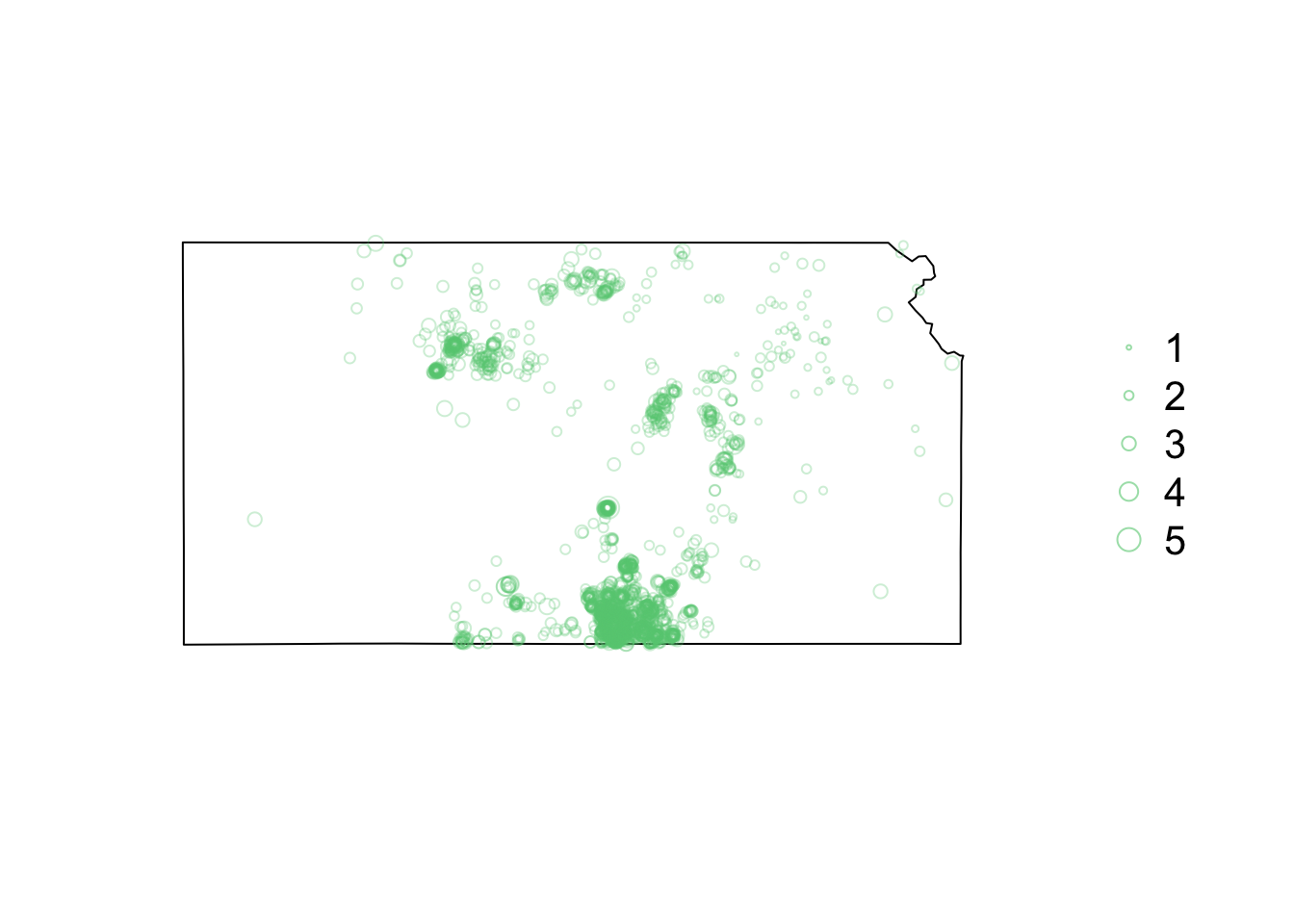
# Plot timeseries of earthquake data
plot(as.numeric(names(table(year(df.eq$Date.time)))), c(table(year(df.eq$Date.time))),
    xlab = "Year", ylab = "Number of Earthquakes in KS", pch = 20)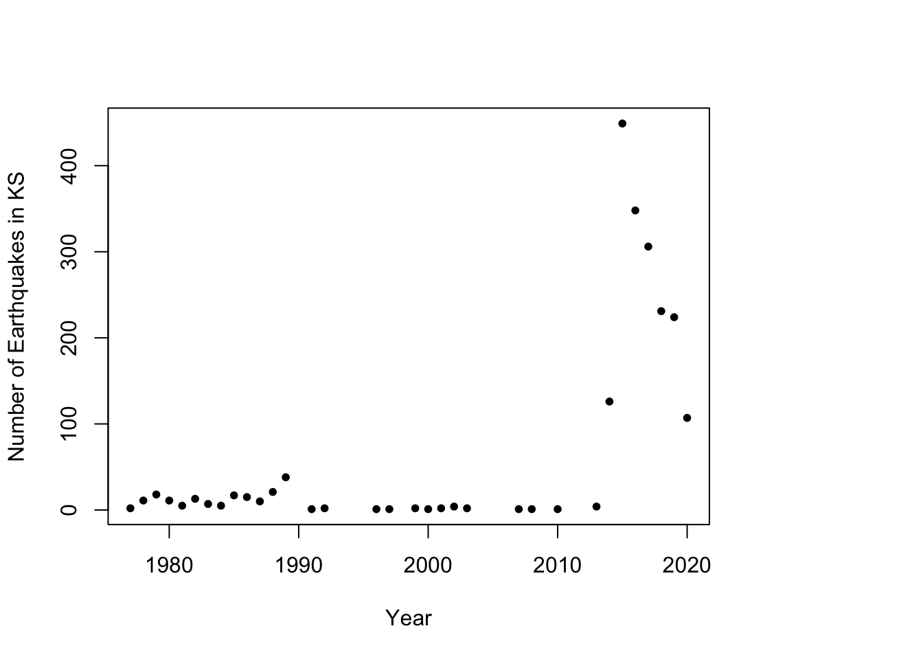
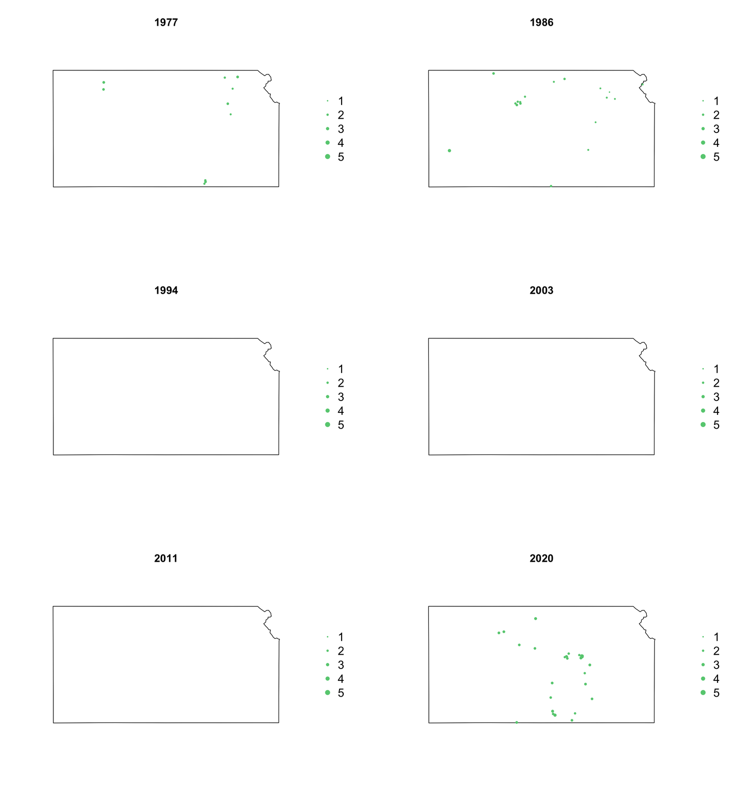
- Animation of Kansas Earthquake data
# Make animation of earthquake data
date <- seq(as.Date("1977-1-1"), as.Date("2020-10-31"), by = "year")
t <- round(time_length(interval(min(date), pts.eq$Date.time), "year"))

for (i in 1:length(date)) {
    par(mar = c(5.1, 4.1, 4.1, 8.1), xpd = TRUE)
    plot(sf.kansas, main = year(date[i]))
    legend("right", inset = c(-0.25, 0), legend = c(1, 2, 3, 4, 5), bty = "n", text.col = "black",
        pch = 20, cex = 1.3, pt.cex = c(1, 2, 3, 4, 5)/3, col = rgb(0.4, 0.8, 0.5,
            1))
    if (length(which(t == i)) > 0) {
        points(pts.eq[which(t == i), ], col = rgb(0.4, 0.8, 0.5, 1), pch = 20, cex = pts.eq[which(t ==
            i), ]$Magnitude/3)
    }
}
21.4 Spatio-temporal models for earthquake data
- What are the goals of our study?
- Prediction
- Make point and areal level predictions
- Inference
- Understand the spatio-temporal covariates that may increase or decrease the risk of an earthquake
- Prediction
- What auxiliary data do we need?
- Kansas oil and gas well data
- Descriptive vs. dynamic approach
- Write out statistical model for earthquake data
- Read this paper (link)