19 Day 19 (March 31)

19.1 Announcements

Office hours today will be from 2-3pm (Dickens Hall room 109)
Office hours on thursday are canceled, but I will have additional hours on Friday from 3-4pm (Dickens Hall room 109)
Calendar is updated
Work day on Thursday (April 2)
- Peer review is due May 1 (ish)
- Report and tutorial are due May 10
- My preference for presentations is May 4-8. Please send me an email (thefley@ksu.edu) and provide three 30 min long times/dates that work for you.
Read this paper (link)
Questions/clarifications from journals
- Model evaluation in parking lot example/Activity 3? (see here)
- “I found the discussion about spatial autocorrelation versus other types of correlation very interesting because I have been wondering about the same issue. In particular, what processes can generate autocorrelation in the data….”
- “What specific designs are commonly used in wildlife studies and how they improve inference compared to the type of observational data we are using? (see here)
- “I am sort of struggling to find how to fit more space and time inference into my project. Since it was a design, the only thing so far is to just add random spatial and temporal terms and call it good.”

19.2 Spatio-temporal models for disease data

Example

Data from Enders et al (2018) which is available on Dryad Digital Repository
Example of my own person “tutorial” link
R code for todays example

library(sf)
library(sp)
library(raster)

url <- "https://www.dropbox.com/scl/fi/9ymxt900s77uq50ca6dgc/Enders-et-al.-2018-data.csv?rlkey=0rxjwleenhgu0gvzow5p0x9xf&dl=1"
df1 <- read.csv(url)
df1 <- df1[, c(1, 4, 5, 8, 9, 10)]  # Keep only the data on bird cherry-oat aphid

head(df1)

##   BCOA BYDV.totalpos.BCOA BCOA.totaltested year      long      lat
## 1   12                  2               10 2014 -95.16269 37.86238
## 2    1                  0                1 2014 -95.28463 38.29669
## 3    2                  0                2 2014 -95.33038 39.59482
## 4    0                 NA                0 2014 -95.32098 39.50696
## 5    8                  0                8 2014 -98.55469 38.48455
## 6    1                  0                1 2014 -98.84792 38.32772

# Download shapefile of Kansas from census.gov
download.file("http://www2.census.gov/geo/tiger/GENZ2015/shp/cb_2015_us_state_20m.zip",
    destfile = "states.zip")
unzip("states.zip")
sf.us <- st_read("cb_2015_us_state_20m.shp", quiet = TRUE)
sf.kansas <- sf.us[48, 6]
sf.kansas <- as(sf.kansas, "Spatial")
# plot(sf.kansas,main='',col='white')

# Make SpatialPoints data frame
pts.sample <- data.frame(long = df1$long, lat = df1$lat, count = df1$BCOA, BYDV.pos = df1$BYDV.totalpos.BCOA,
    BYDV.tot = df1$BCOA.totaltested, BYDV.prop = df1$BYDV.totalpos.BCOA/df1$BCOA.totaltested)
coordinates(pts.sample) = ~long + lat
proj4string(pts.sample) <- CRS("+proj=longlat +datum=WGS84 +no_defs +ellps=WGS84 +towgs84=0,0,0")


# Plot counts of Bird cherry-oat aphid
par(mar = c(5.1, 4.1, 4.1, 8.1), xpd = TRUE)
plot(sf.kansas, main = "Abundance of Bird Cherry-oat Aphid")
points(pts.sample[, 1], col = rgb(0.4, 0.8, 0.5, 0.9), pch = ifelse(pts.sample$count >
    0, 20, 4), cex = pts.sample$count/50 + 0.5)
legend("right", inset = c(-0.25, 0), legend = c(0, 1, 10, 20, 40, 60), bty = "n",
    text.col = "black", pch = c(4, 20, 20, 20, 20, 20), cex = 1.3, pt.cex = c(0,
        1, 10, 20, 40, 60)/50 + 0.5, col = rgb(0.4, 0.8, 0.5, 0.9))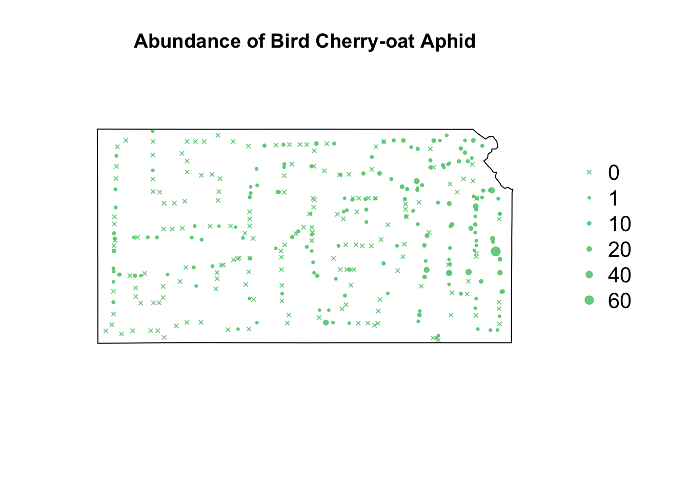

# Plot proportion of number of Bird cherry-oat aphid infected with BYDV
par(mar = c(5.1, 4.1, 4.1, 8.1), xpd = TRUE)
plot(sf.kansas, main = "Proportion infected")
points(pts.sample[, 4], col = rgb(0.8, 0.5, 0.4, 0.9), pch = ifelse(is.na(pts.sample$BYDV.prop) ==
    FALSE, 20, 4), cex = ifelse(is.na(pts.sample$BYDV.prop) == FALSE, pts.sample$BYDV.prop,
    0)/0.5 + 0.5)
legend("right", inset = c(-0.25, 0), legend = c("NA", 0, 0.25, 0.5, 0.75, 1), bty = "n",
    text.col = "black", pch = c(4, 20, 20, 20, 20, 20), cex = 1.3, pt.cex = c(0,
        0, 0.25, 0.5, 0.75, 1)/0.5 + 0.5, col = rgb(0.8, 0.5, 0.4, 0.9))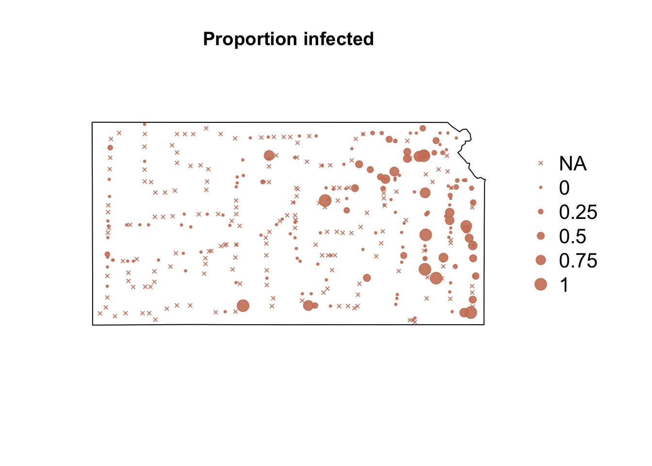

Study goals
- Make accurate predictions of vector abundance and probability of BYDV infection at times and locations where data was not collected.
- Understand the environmental factors (e.g., temperature) that influence the vector abundance and probability of BYDV infection.
Auxiliary data
- Weather/climate data
- Land cover data
- Crop data
Model choice: dynamic vs. descriptive spatio-temporal model?
- Class discussion
Next steps
- Write out the statistical model(s)
- Determine how we will evaluate how model(s)
- Determine how we will make inference

19.3 Earthquake data

New York Times article
New York Times articles

Earthquake data from Kansas

library(sf)
library(sp)
library(raster)
library(lubridate)
library(animation)
library(gifski)


# Download shapefile of Kansas from census.gov
download.file("http://www2.census.gov/geo/tiger/GENZ2015/shp/cb_2015_us_state_20m.zip",
    destfile = "states.zip")
unzip("states.zip")
sf.us <- st_read("cb_2015_us_state_20m.shp", quiet = TRUE)
sf.kansas <- sf.us[48, 6]
sf.kansas <- as(sf.kansas, "Spatial")

# Load earthquake data
url <- "https://www.dropbox.com/scl/fi/uhicc7qo4zcxeq79y1eh9/ks_earthquake_data.csv?rlkey=lbq8kxzx9g067domp46ffh7jw&dl=1"
df.eq <- read.csv(url)
df.eq$Date.time <- ymd_hms(df.eq$Date.time)
pts.eq <- SpatialPointsDataFrame(coords = df.eq[, c(3, 2)], data = df.eq[, c(1, 4)],
    proj4string = crs(sf.kansas))

# Plot spatial map earthquake data
par(mar = c(5.1, 4.1, 4.1, 8.1), xpd = TRUE)
plot(sf.kansas, main = "")
points(pts.eq, col = rgb(0.4, 0.8, 0.5, 0.3), pch = 21, cex = pts.eq$Magnitude/3)
legend("right", inset = c(-0.25, 0), legend = c(1, 2, 3, 4, 5), bty = "n", text.col = "black",
    pch = 21, cex = 1.3, pt.cex = c(1, 2, 3, 4, 5)/3, col = rgb(0.4, 0.8, 0.5, 0.6))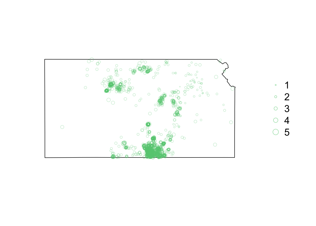

# Plot timeseries of earthquake data
plot(as.numeric(names(table(year(df.eq$Date.time)))), c(table(year(df.eq$Date.time))),
    xlab = "Year", ylab = "Number of Earthquakes in KS", pch = 20)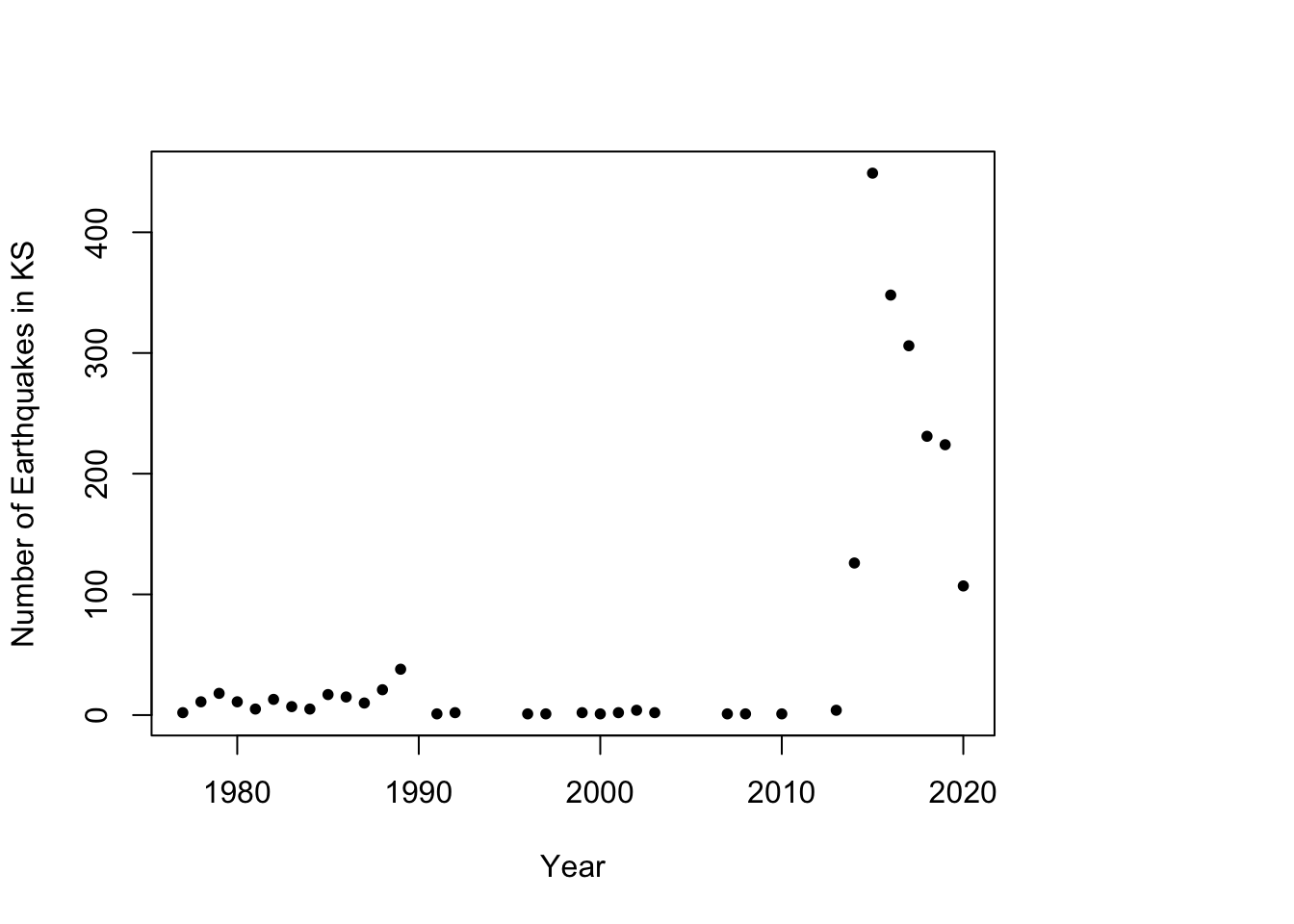

Animation of Kansas Earthquake data

# Make animation of earthquake data
date <- seq(as.Date("1977-1-1"), as.Date("2020-10-31"), by = "year")
t <- round(time_length(interval(min(date), pts.eq$Date.time), "year"))

for (i in 1:length(date)) {
    par(mar = c(5.1, 4.1, 4.1, 8.1), xpd = TRUE)
    plot(sf.kansas, main = year(date[i]))
    legend("right", inset = c(-0.25, 0), legend = c(1, 2, 3, 4, 5), bty = "n", text.col = "black",
        pch = 20, cex = 1.3, pt.cex = c(1, 2, 3, 4, 5)/3, col = rgb(0.4, 0.8, 0.5,
            1))
    if (length(which(t == i)) > 0) {
        points(pts.eq[which(t == i), ], col = rgb(0.4, 0.8, 0.5, 1), pch = 20, cex = pts.eq[which(t ==
            i), ]$Magnitude/3)
    }
}

19.4 Spatio-temporal models for earthquake data

What are the goals of our study?
- Prediction
  - Make point and areal level predictions
- Inference
  - Understand the spatio-temporal covariates that may increase or decrease the risk of an earthquake
What auxiliary data do we need?
Kansas oil and gas well data
Descriptive vs. dynamic approach
Write out statistical model for earthquake data
Read this paper (link)