7 Day 7 (February 10)

7.1 Announcements

Donuts on Thursday
- About 20-30 min at end of class to meet your peers!
Read and re-read pgs. 10-14 of Spatio-temporal statistics with R.
- Review distribution theory notes
- Review mathematical modeling notes
Questions/clarifications from journals
- “Can agent-based models account for uncertainty? Or are they purely deterministic?” (see here)
- “Today I learned that statistical results don’t come directly from the data alone, they come from the assumptions we build into a model….Overall, I’m starting to see modeling less as picking a method and more as building a reasonable set of assumptions for the situation.”
- “In agronomic data, including random factors often feels conceptually reasonable, but I am not clear on how to evaluate whether the added structure is truly improving the model or simply introducing bias through additional assumptions. For example, if a random effect seems biologically meaningful, is that alone enough reason to include it, or should the decision be based on statistical criteria?”

7.1.1 Motivating data example

Whooping cranes

Data set

url <- "https://www.dropbox.com/scl/fi/kxzc8fmomkigcrxyjjmdp/Butler-et-al.-Table-1.csv?rlkey=61ey3q1jc4rsor257uy4080j3&dl=1"
df1 <- read.csv(url)

plot(df1$Winter, df1$N, xlab = "Year", ylab = "Population count (z)", xlim = c(1940,
    2020), ylim = c(0, 300), typ = "b", cex = 0.8, pch = 20, col = rgb(0.7, 0.7,
    0.7, 0.9))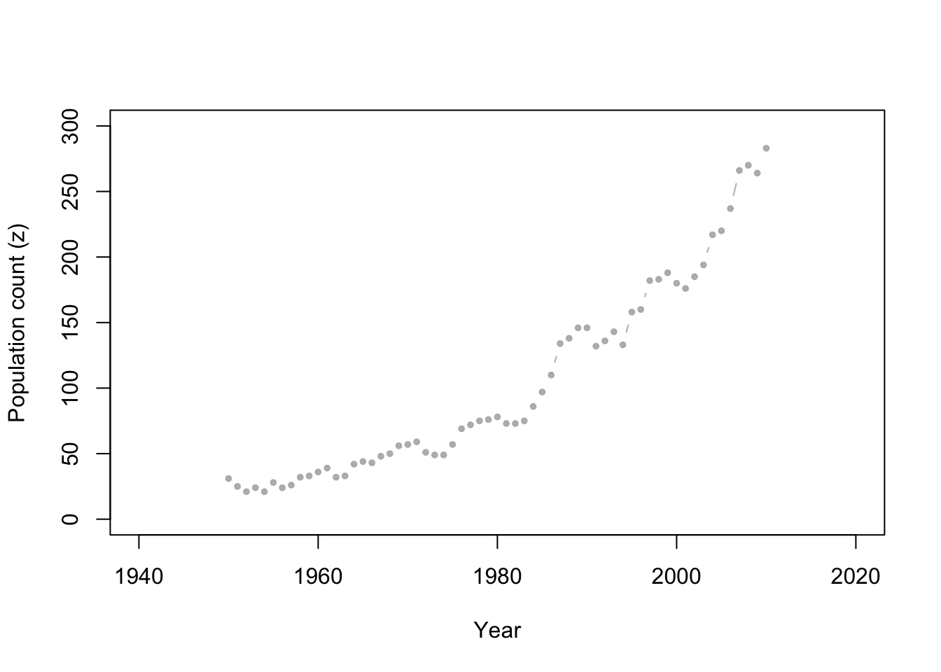

Live example Download R code here
We want to build a statistical model that enables
- Predictions and forecasts of the true population size
- Statistical inference on the date when the population will be larger than 1000 individuals
Points to consider
- Whooping cranes are counted from an airplane (could some individuals be missed?)
- Aggregation of a spatio-temporal point pattern?
- Are there any existing models that could work for these data?
- Anything else?
Mathematical model for whooping crane data
- Ordinary differential equations
- The expected number of whooping cranes at any given time can be calculated by\[\lambda(t+\Delta t)=\lambda(t)+b(t)-d(t)\:.\]At time t, let the births equal \(b(t)=\beta\Delta t\lambda(t)\) and deaths equal \(d(t)=\alpha\Delta t\lambda(t)\). Then write the equation above as \[\lambda(t+\Delta t)=\lambda(t)+\beta\Delta t\lambda(t)-\alpha\Delta t\lambda(t)\:.\] Now define the growth rate as \(\gamma=\beta-\alpha\) and rewrite as \[\lambda(t+\Delta t)=\lambda(t)+\gamma\Delta t\lambda(t)\:.\] Next write the equation as\[\frac{\lambda(t+\Delta t)-\lambda(t)}{\Delta t}=\gamma\lambda(t)\] and let \[\Delta t\rightarrow0\lim_{\Delta t\rightarrow0}\frac{\lambda(t+\Delta t)-\lambda(t)}{\Delta t}=\gamma\lambda(t)\:.\] Finally replace \(\lim_{\Delta t\rightarrow0}\frac{\lambda(t+\Delta t)-\lambda(t)}{\Delta t}\) with the differential operator\[\frac{d\lambda(t)}{dt}=\gamma\lambda(t)\:.\]
- Solving requires an ODE and initial conditions
  - The expected number of whooping cranes in 1949?
- Analytical solution to ODEs \[\lambda(t)=\lambda_{0}e^{\gamma t}\]
- Numerical solution to ODEs
  - Finite difference method (replace \(\frac{d\lambda(t)}{dt}\) with \(\frac{\lambda_{t+\Delta t}-\lambda_{t}}{\Delta t}\)) \[\frac{d\lambda(t)}{dt}=\gamma\lambda\] \[\frac{\lambda_{t+\Delta t}-\lambda_{t}}{\Delta t}=\gamma\lambda\] \[\lambda_{t+\Delta t}=\lambda_{t}+\gamma\Delta t\lambda_{t}\]

7.2 Hierarchical models

During this course we will implement many models using the hierarchical framework
- Hierarchical models are pretty common (e.g., mixed models, kriging, most Bayesian models)
- Today is a crash course on hierarchical and Bayesian statistical models
- Study technical note 1.1 on pg. 13 of Spatio-temporal statistics with R
The Bayesian hierarchical modeling framework

\[\text{Data model:} \;\;[\mathbf{z}|\mathbf{y},\boldsymbol{\theta}_{D}]\] \[\text{Process model:} \;\;[\mathbf{y}|\boldsymbol{\theta}_{P}]\] \[\text{Parameter model:} \;\;[\boldsymbol{\theta}]\]