13 Day 13 (March 3)

13.1 Announcements

Thursday will be a workday. There is no journal due, but if you’d like to submit one, please do. I will be gone for the first half of class.
Read Ch. 4 pgs 137-192
- Concepts and Synthesis paper
Questions/clarifications from journals
- “Something that feels obvious: if latitude and longitude jointly define spatial location, then their interaction should probably be included from the start. Modeling them only as additive effects feels like an oversimplification of spatial structure. I find it hard to reconcile this simplification with the intuitive idea of spatial dependence.”
- “I’ve been struggling to understand how much emphasis we should place on model diagnostics in spatio-temporal statistics. In class we’ve fitted some models (for example, the whooping cranes example, a car-related example, and the coin-flip example), but I didn’t see us go through the usual checks I’m used to from regression things like checking assumptions, linearity, constant variance, independence, and residual patterns. This made me wonder whether these diagnostics are less necessary in spatio-temporal models?”
- “I was a little bit confused when we discussed the practice of averaging your data. I understand this is a form of data destruction, but is it sometimes necessary for an analysis?”
Activity 3 is due sometime next week… Dickens Hall parking lot example

13.2 Extreme precipitation in Kansas

Note, this is essentially the same as activity 2
On September 3, 2018 there was an extreme precipitation event that resulted in flooding in Manhattan, KS and the surrounding areas. If you would like to know more about this, check out this link and this video here and here.
My process
- Determine the goals of the study
- Data acquisition
  - Live demonstration (Download R code here)
- Exploratory data analysis
  - Live demonstration
- The model building process
  - 1). Choose appropriate PDFs or PMFs for the data, process, and parameter models
  - 2). Choose appropriate mathematical models for the “parameters” or moments of the PDFs/PMFs from step 1.
  - 3). Choose an algorithm fit the statistical model to the data
  - 4). Make statistical inference (e.g., calculate derived quantities and summarize the posterior distribution)
- Model checking, improvements, validation, and selection (Ch. 6)
What we will need to learn
- How to use R as a geographic information system
- New general tools from statistics
  - Gaussian process
  - Metropolis and Metropolis–Hastings algorithms
  - Gibbs sampler
- How to use the hierarchical modeling framework to describe Kriging
  - Hierarchical Bayesian model vs. “empirical” hierarchical model
- Specialized language used in spatial statistics (e.g., range, nugget, variogram)

13.3 Linear models for correlated errors

Motivating example

Regression/polynomial example Download R code here

ISIT <- read.table("https://www.dropbox.com/scl/fi/n5ku9crpsr384p9z2rc8b/bioluminescence.txt?rlkey=airzs2ukql4g0hqxjr72re53j&dl=1",
    header = TRUE)

Sources16 <- ISIT$Sources[ISIT$Station == 16]
Depth16 <- ISIT$SampleDepth[ISIT$Station == 16]
Sources16 <- Sources16[order(Depth16)]
Depth16 <- sort(Depth16)
plot(Depth16, Sources16, las = 1, ylim = c(0, 65), col = rgb(0, 0, 0, 0.25), pch = 19,
    ylab = "Density of bioluminescence", xlab = "Depth in meters")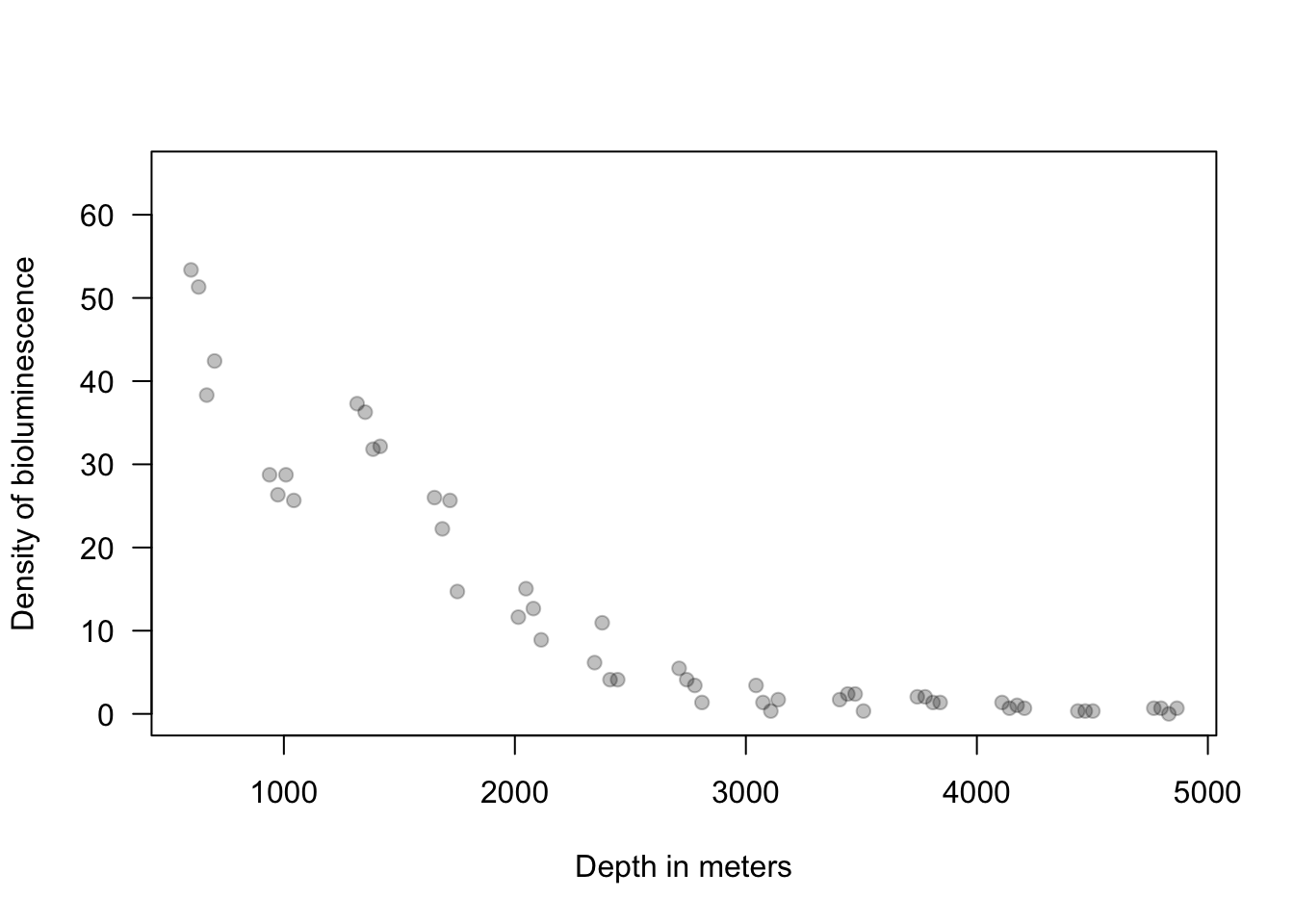

Linear model with correlated errors (aka Kriging)
- \(\mathbf{\textbf{y}}=\mathbf{X}\boldsymbol{\beta}+\boldsymbol{\eta}+\boldsymbol{\varepsilon}\) where \(\boldsymbol{\eta}\sim\text{N}(\mathbf{0},\sigma_{\eta}^{2}\mathbf{R}(\phi))\) and \(\boldsymbol{\varepsilon}\sim\text{N}(\mathbf{0},\sigma_{\varepsilon}^{2}\mathbf{I})\)
- The model above is the same as \(\mathbf{y}\sim\text{N}(\mathbf{X}\boldsymbol{\beta},\sigma_{\eta}^{2}\mathbf{R}(\phi)+\sigma^{2}\mathbf{I})\)
- Estimation
  - Regression coefficients \[\hat{\boldsymbol{\beta}}=(\mathbf{X}^{\prime}\mathbf{V}^{-1}\mathbf{X})^{-1}\mathbf{X}^{\prime}\mathbf{V}^{-1}\mathbf{y}\] where \(\mathbf{V=}\sigma_{\eta}^{2}\mathbf{R}(\phi)+\sigma_{\varepsilon}^{2}\mathbf{I}\)
  - Numerical maximization to estimate \(\sigma_{\eta}^{2}\), \(\sigma^{2}\), and \(\phi\)
- Error terms \[\hat{\boldsymbol{\eta}}=\hat{\sigma}_{\eta}^{2}\mathbf{R}(\hat{\phi})(\hat{\sigma}_{\varepsilon}^{2}\mathbf{I}+\hat{\sigma}_{\eta}^{2}\mathbf{R}(\hat{\phi}))^{-1}(\mathbf{y}-\mathbf{X}\hat{\boldsymbol{\beta}})\] \[\hat{\boldsymbol{\varepsilon}} = \mathbf{y} - \mathbf{X}\hat{\boldsymbol{\beta}} - \hat{\boldsymbol{\eta}}\]

Bioluminescence example

Intercept only linear model

ISIT <- read.table("https://www.dropbox.com/scl/fi/n5ku9crpsr384p9z2rc8b/bioluminescence.txt?rlkey=airzs2ukql4g0hqxjr72re53j&dl=1",
    header = TRUE)

Sources16 <- ISIT$Sources[ISIT$Station == 16]
Depth16 <- ISIT$SampleDepth[ISIT$Station == 16]
Sources16 <- Sources16[order(Depth16)]
Depth16 <- sort(Depth16)

m1 <- lm(Sources16 ~ 1)
e.hat.m1 <- residuals(m1)

plot(Depth16, e.hat.m1, xlab = "Depth (m)", ylab = expression(hat(epsilon)), ylim = c(-15,
    60), las = 1, col = rgb(0, 0, 0, 0.25))
abline(a = 0, b = 0)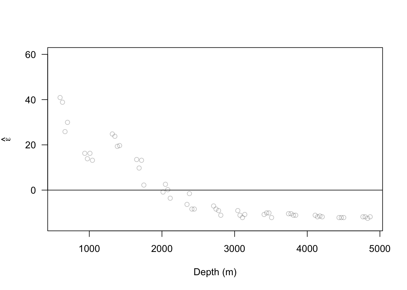

Intercept only linear model with spatial random effect

library(nlme)
m2 <- gls(Sources16 ~ 1, correlation = corGaus(form = ~Depth16, nugget = TRUE, value = c(100,
    0.05), fixed = FALSE), method = "ML")

summary(m2)

## Generalized least squares fit by maximum likelihood
##   Model: Sources16 ~ 1 
##   Data: NULL 
##        AIC      BIC    logLik
##   296.3003 304.0276 -144.1502
## 
## Correlation Structure: Gaussian spatial correlation
##  Formula: ~Depth16 
##  Parameter estimate(s):
##        range       nugget 
## 610.73574379   0.01300607 
## 
## Coefficients:
##                Value Std.Error  t-value p-value
## (Intercept) 17.73824  8.981483 1.974978  0.0538
## 
## Standardized residuals:
##        Min         Q1        Med         Q3        Max 
## -0.8937320 -0.8247052 -0.6866517  0.3991341  1.7952883 
## 
## Residual standard error: 19.84738 
## Degrees of freedom: 51 total; 50 residual

# estimated range & nugget parameters from gls
phi <- exp(m2$model[1]$corStruct[1])^2
nugget <- 1/(1 + exp(-m2$model[1]$corStruct[2]))


X <- rep(1, length(Sources16))
y <- Sources16

sigma2.eta <- (m2$sigma^2) * (1 - nugget)
R <- exp(-as.matrix(dist(Depth16, diag = TRUE, upper = TRUE))^2/phi)
sigma2.e <- (m2$sigma^2) * nugget
I <- diag(1, length(y))
V <- sigma2.eta * R + sigma2.e * I
beta <- solve(t(X) %*% solve(V) %*% X) %*% t(X) %*% solve(V) %*% y

eta <- sigma2.eta * R %*% solve(V) %*% (y - X %*% beta)

par(mar = c(5.1, 4.1, 2.1, 2.1), oma = c(0, 0, 0, 0))  # reset plot margins
par(mfrow = c(1, 2))  # plot layout
par(pch = 19)  # plotting symbol

# plot predictions for second-order spatial model
plot(Depth16, Sources16, xlab = "Depth (m)", ylab = "Density of bioluminescence",
    ylim = c(-15, 60), las = 1, col = rgb(0, 0, 0, 0.25))
lines(Depth16, X %*% beta + eta, col = "black")
lines(Depth16, X %*% beta, col = "purple")

e.hat.m2 <- y - (X %*% beta + eta)
plot(Depth16, e.hat.m2, xlab = "Depth (m)", ylab = expression(hat(epsilon)), las = 1,
    col = rgb(0, 0, 0, 0.25))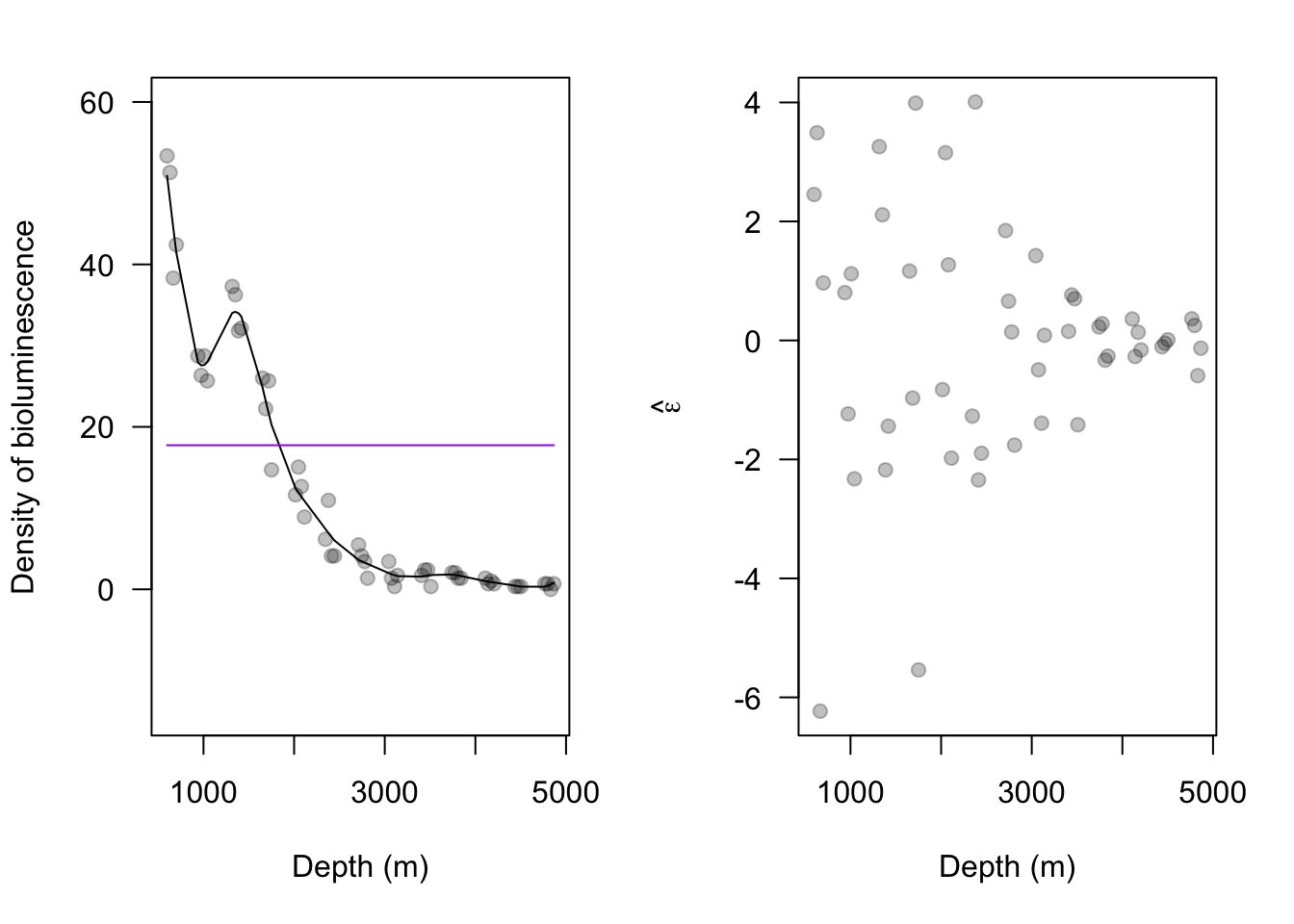

Homework assignment!
- Go back to the R code for the bioluminescence example and allow the expected value of bioluminescence density to depend on depth (i.e., use a linear model with a slope parameter instead of just an intercept)

13.4 Extreme precipitation in Kansas

Let’s try to use what we have learned to make a better model
- Live demonstration (Download R code here)