15 Day 15 (March 10)
15.1 Announcements
Read Ch. 4 pgs 137-192
Activity 3 is due Friday at 11:59pm Dickens Hall parking lot example
Questions/clarifications from journals
- Spatio-temporal models for spatial data (link)

- “One thing I am still struggling to understand is when modeling assumptions can be overlooked. My prior knowledge about linear models is that the residuals should have constant variance or should appear random without any specific pattern. But in the bioluminescence example in class, the residual plot appeared to have a funnel pattern, and you seemed okay with the model. Can we ignore some assumptions in model fitting?”
- “In the bioluminescence example, does the parameter \(\phi\) control how quickly correlation decreases as depth separation increases? Also, does the nugget represent microscale variation or measurement error that is not smooth?”
- “My main concern is: what if I do most of my analysis first, then check spatial correlation and find it’s weak or not significant (or the nugget dominates)? Do I just simplify to an independent-error model and explain that the data doesn’t support strong correlation? Or does “no correlation” mean I used the wrong scale, missed key predictors, or I should be checking correlation in the residuals instead of the raw outcome?”
- Spatio-temporal models for spatial data (link)
15.2 Extreme precipitation in Kansas
- Let’s try to use what we have learned to make a better model
- Live demonstration (Download R code here)
- Wrap-up of this example
- What we accomplished
- Point predictions of rainfall amounts at any location within the study area.
- Estimated the maximum amount of rainfall within the study area and the location where it fell
- What we did not accomplished
- Uncertainty quantification!
- Would need to use MC or MCMC-based methods.
- What we accomplished
15.3 Spatio-temporal models for disease data
Example
- Data from Enders et al (2018) which is available on Dryad Digital Repository
library(sf)
library(sp)
library(raster)

url <- "https://www.dropbox.com/scl/fi/9ymxt900s77uq50ca6dgc/Enders-et-al.-2018-data.csv?rlkey=0rxjwleenhgu0gvzow5p0x9xf&dl=1"
df1 <- read.csv(url)
df1 <- df1[, c(1, 4, 5, 8, 9, 10)]  # Keep only the data on bird cherry-oat aphid

head(df1)
## BCOA BYDV.totalpos.BCOA BCOA.totaltested year long lat ## 1 12 2 10 2014 -95.16269 37.86238 ## 2 1 0 1 2014 -95.28463 38.29669 ## 3 2 0 2 2014 -95.33038 39.59482 ## 4 0 NA 0 2014 -95.32098 39.50696 ## 5 8 0 8 2014 -98.55469 38.48455 ## 6 1 0 1 2014 -98.84792 38.32772# Download shapefile of Kansas from census.gov download.file("http://www2.census.gov/geo/tiger/GENZ2015/shp/cb_2015_us_state_20m.zip", destfile = "states.zip") unzip("states.zip") sf.us <- st_read("cb_2015_us_state_20m.shp", quiet = TRUE) sf.kansas <- sf.us[48, 6] sf.kansas <- as(sf.kansas, "Spatial") # plot(sf.kansas,main='',col='white') # Make SpatialPoints data frame pts.sample <- data.frame(long = df1$long, lat = df1$lat, count = df1$BCOA, BYDV.pos = df1$BYDV.totalpos.BCOA, BYDV.tot = df1$BCOA.totaltested, BYDV.prop = df1$BYDV.totalpos.BCOA/df1$BCOA.totaltested) coordinates(pts.sample) = ~long + lat proj4string(pts.sample) <- CRS("+proj=longlat +datum=WGS84 +no_defs +ellps=WGS84 +towgs84=0,0,0") # Plot counts of Bird cherry-oat aphid par(mar = c(5.1, 4.1, 4.1, 8.1), xpd = TRUE) plot(sf.kansas, main = "Abundance of Bird Cherry-oat Aphid") points(pts.sample[, 1], col = rgb(0.4, 0.8, 0.5, 0.9), pch = ifelse(pts.sample$count > 0, 20, 4), cex = pts.sample$count/50 + 0.5) legend("right", inset = c(-0.25, 0), legend = c(0, 1, 10, 20, 40, 60), bty = "n", text.col = "black", pch = c(4, 20, 20, 20, 20, 20), cex = 1.3, pt.cex = c(0, 1, 10, 20, 40, 60)/50 + 0.5, col = rgb(0.4, 0.8, 0.5, 0.9))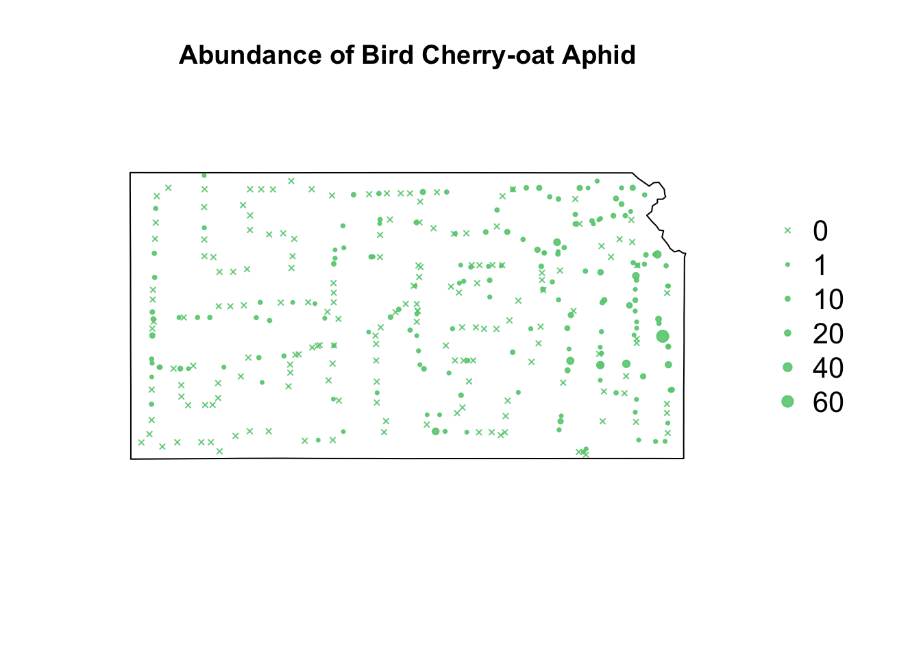
# Plot proportion of number of Bird cherry-oat aphid infected with BYDV
par(mar = c(5.1, 4.1, 4.1, 8.1), xpd = TRUE)
plot(sf.kansas, main = "Proportion infected")
points(pts.sample[, 4], col = rgb(0.8, 0.5, 0.4, 0.9), pch = ifelse(is.na(pts.sample$BYDV.prop) ==
    FALSE, 20, 4), cex = ifelse(is.na(pts.sample$BYDV.prop) == FALSE, pts.sample$BYDV.prop,
    0)/0.5 + 0.5)
legend("right", inset = c(-0.25, 0), legend = c("NA", 0, 0.25, 0.5, 0.75, 1), bty = "n",
    text.col = "black", pch = c(4, 20, 20, 20, 20, 20), cex = 1.3, pt.cex = c(0,
        0, 0.25, 0.5, 0.75, 1)/0.5 + 0.5, col = rgb(0.8, 0.5, 0.4, 0.9))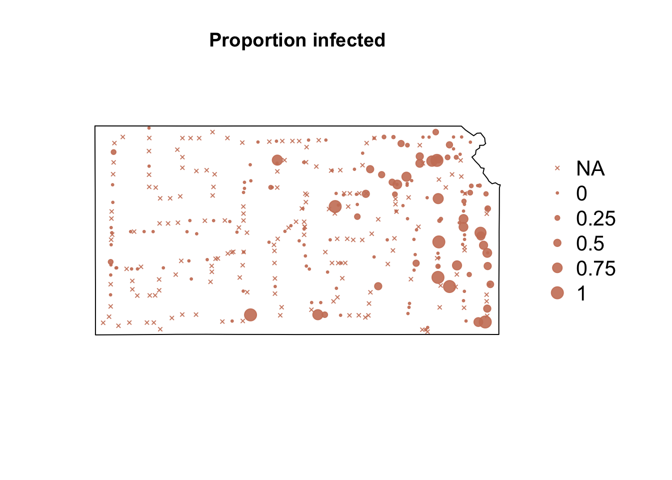
Study goals
- Make accurate predictions of vector abundance and probability of BYDV infection at times and locations where data was not collected.
- Understand the environmental factors (e.g., temperature) that influence the vector abundance and probability of BYDV infection.
Auxiliary data
- Weather/climate data
- Land cover data
- Crop data
Model choice: dynamic vs. descriptive spatio-temporal model?
- Class discussion
Next steps
- Write out the statistical model(s)
- Determine how we will evaluate how model(s)
- Determine how we will make inference