18 Day 18 (March 26)
18.1 Announcements
ASA DataFest mentors needed (link)
Work day next Thursday (April 2)
- Peer review is due May 1 (ish)
- Report and tutorial are due May 10
- My preference for presentations is May 4-8. Please send me an email (thefley@ksu.edu) and provide three 30 min long times/dates that work for you.
Questions/clarifications from journals
- Original work on kernel averaged predictors (see here and here)
- “How do I decide between a dynamic spatio-temporal model and a more descriptive model?”
- “One thing I’m still struggling with is the idea of spatial autocorrelation vs other autocorrelation.”
- “Something related do the class project and also other studies I work with: In field studies with multiple sites where we are using precipitation data, would it be better to use the precipitation measured at the weather station closest to each site, or would it be more appropriate to use data from multiple surrounding stations to model precipitation spatially and estimate rainfall at each site?”
18.2 Spatio-temporal models for disease data
Example
- Data from Enders et al (2018) which is available on Dryad Digital Repository
- Example of my own person “tutorial” link
- R code for todays example
library(sf)
library(sp)
library(raster)

url <- "https://www.dropbox.com/scl/fi/9ymxt900s77uq50ca6dgc/Enders-et-al.-2018-data.csv?rlkey=0rxjwleenhgu0gvzow5p0x9xf&dl=1"
df1 <- read.csv(url)
df1 <- df1[, c(1, 4, 5, 8, 9, 10)]  # Keep only the data on bird cherry-oat aphid

head(df1)
## BCOA BYDV.totalpos.BCOA BCOA.totaltested year long lat ## 1 12 2 10 2014 -95.16269 37.86238 ## 2 1 0 1 2014 -95.28463 38.29669 ## 3 2 0 2 2014 -95.33038 39.59482 ## 4 0 NA 0 2014 -95.32098 39.50696 ## 5 8 0 8 2014 -98.55469 38.48455 ## 6 1 0 1 2014 -98.84792 38.32772# Download shapefile of Kansas from census.gov download.file("http://www2.census.gov/geo/tiger/GENZ2015/shp/cb_2015_us_state_20m.zip", destfile = "states.zip") unzip("states.zip") sf.us <- st_read("cb_2015_us_state_20m.shp", quiet = TRUE) sf.kansas <- sf.us[48, 6] sf.kansas <- as(sf.kansas, "Spatial") # plot(sf.kansas,main='',col='white') # Make SpatialPoints data frame pts.sample <- data.frame(long = df1$long, lat = df1$lat, count = df1$BCOA, BYDV.pos = df1$BYDV.totalpos.BCOA, BYDV.tot = df1$BCOA.totaltested, BYDV.prop = df1$BYDV.totalpos.BCOA/df1$BCOA.totaltested) coordinates(pts.sample) = ~long + lat proj4string(pts.sample) <- CRS("+proj=longlat +datum=WGS84 +no_defs +ellps=WGS84 +towgs84=0,0,0") # Plot counts of Bird cherry-oat aphid par(mar = c(5.1, 4.1, 4.1, 8.1), xpd = TRUE) plot(sf.kansas, main = "Abundance of Bird Cherry-oat Aphid") points(pts.sample[, 1], col = rgb(0.4, 0.8, 0.5, 0.9), pch = ifelse(pts.sample$count > 0, 20, 4), cex = pts.sample$count/50 + 0.5) legend("right", inset = c(-0.25, 0), legend = c(0, 1, 10, 20, 40, 60), bty = "n", text.col = "black", pch = c(4, 20, 20, 20, 20, 20), cex = 1.3, pt.cex = c(0, 1, 10, 20, 40, 60)/50 + 0.5, col = rgb(0.4, 0.8, 0.5, 0.9))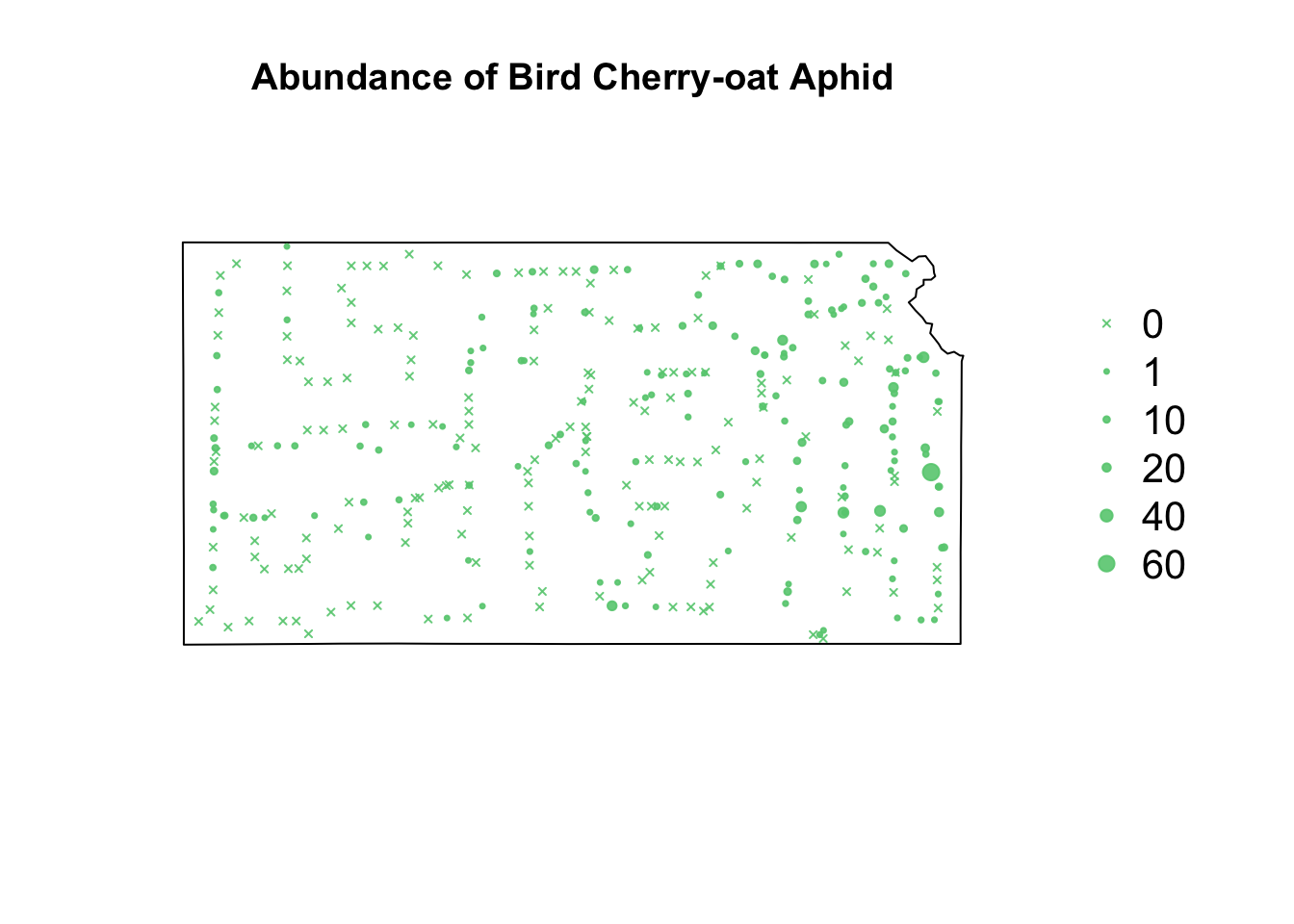
# Plot proportion of number of Bird cherry-oat aphid infected with BYDV
par(mar = c(5.1, 4.1, 4.1, 8.1), xpd = TRUE)
plot(sf.kansas, main = "Proportion infected")
points(pts.sample[, 4], col = rgb(0.8, 0.5, 0.4, 0.9), pch = ifelse(is.na(pts.sample$BYDV.prop) ==
    FALSE, 20, 4), cex = ifelse(is.na(pts.sample$BYDV.prop) == FALSE, pts.sample$BYDV.prop,
    0)/0.5 + 0.5)
legend("right", inset = c(-0.25, 0), legend = c("NA", 0, 0.25, 0.5, 0.75, 1), bty = "n",
    text.col = "black", pch = c(4, 20, 20, 20, 20, 20), cex = 1.3, pt.cex = c(0,
        0, 0.25, 0.5, 0.75, 1)/0.5 + 0.5, col = rgb(0.8, 0.5, 0.4, 0.9))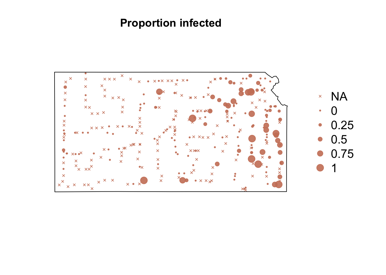
Study goals
- Make accurate predictions of vector abundance and probability of BYDV infection at times and locations where data was not collected.
- Understand the environmental factors (e.g., temperature) that influence the vector abundance and probability of BYDV infection.
Auxiliary data
- Weather/climate data
- Land cover data
- Crop data
Model choice: dynamic vs. descriptive spatio-temporal model?
- Class discussion
Next steps
- Write out the statistical model(s)
- Determine how we will evaluate how model(s)
- Determine how we will make inference
18.3 Earthquake data
-
library(sf)
library(sp)
library(raster)
library(lubridate)
library(animation)
library(gifski)


# Download shapefile of Kansas from census.gov
download.file("http://www2.census.gov/geo/tiger/GENZ2015/shp/cb_2015_us_state_20m.zip",
    destfile = "states.zip")
unzip("states.zip")
sf.us <- st_read("cb_2015_us_state_20m.shp", quiet = TRUE)
sf.kansas <- sf.us[48, 6]
sf.kansas <- as(sf.kansas, "Spatial")

# Load earthquake data
url <- "https://www.dropbox.com/scl/fi/uhicc7qo4zcxeq79y1eh9/ks_earthquake_data.csv?rlkey=lbq8kxzx9g067domp46ffh7jw&dl=1"
df.eq <- read.csv(url)
df.eq$Date.time <- ymd_hms(df.eq$Date.time)
pts.eq <- SpatialPointsDataFrame(coords = df.eq[, c(3, 2)], data = df.eq[, c(1, 4)],
    proj4string = crs(sf.kansas))

# Plot spatial map earthquake data
par(mar = c(5.1, 4.1, 4.1, 8.1), xpd = TRUE)
plot(sf.kansas, main = "")
points(pts.eq, col = rgb(0.4, 0.8, 0.5, 0.3), pch = 21, cex = pts.eq$Magnitude/3)
legend("right", inset = c(-0.25, 0), legend = c(1, 2, 3, 4, 5), bty = "n", text.col = "black",
    pch = 21, cex = 1.3, pt.cex = c(1, 2, 3, 4, 5)/3, col = rgb(0.4, 0.8, 0.5, 0.6))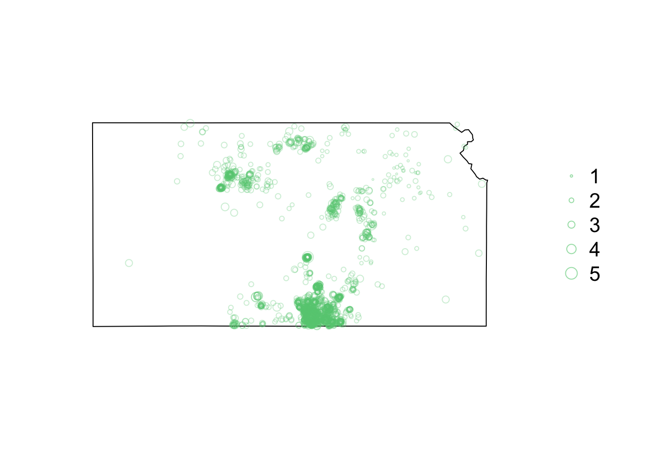
# Plot timeseries of earthquake data
plot(as.numeric(names(table(year(df.eq$Date.time)))), c(table(year(df.eq$Date.time))),
    xlab = "Year", ylab = "Number of Earthquakes in KS", pch = 20)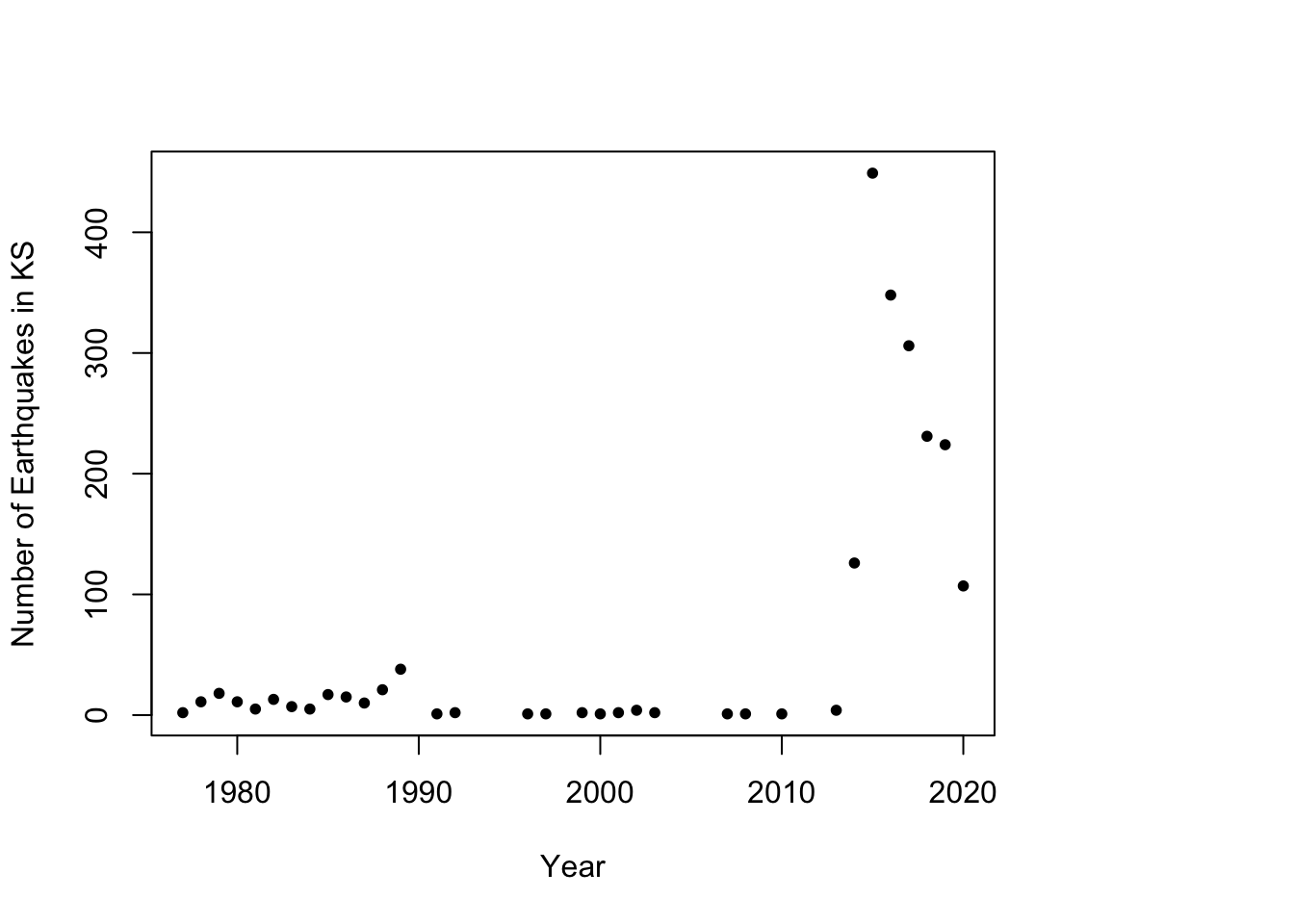
- Animation of Kansas Earthquake data
# Make animation of earthquake data
date <- seq(as.Date("1977-1-1"), as.Date("2020-10-31"), by = "year")
t <- round(time_length(interval(min(date), pts.eq$Date.time), "year"))

for (i in 1:length(date)) {
    par(mar = c(5.1, 4.1, 4.1, 8.1), xpd = TRUE)
    plot(sf.kansas, main = year(date[i]))
    legend("right", inset = c(-0.25, 0), legend = c(1, 2, 3, 4, 5), bty = "n", text.col = "black",
        pch = 20, cex = 1.3, pt.cex = c(1, 2, 3, 4, 5)/3, col = rgb(0.4, 0.8, 0.5,
            1))
    if (length(which(t == i)) > 0) {
        points(pts.eq[which(t == i), ], col = rgb(0.4, 0.8, 0.5, 1), pch = 20, cex = pts.eq[which(t ==
            i), ]$Magnitude/3)
    }
}
18.4 Spatio-temporal models for earthquake data
- What are the goals of our study?
- Prediction
- Make point and areal level predictions
- Inference
- Understand the spatio-temporal covariates that may increase or decrease the risk of an earthquake
- Prediction
- What auxiliary data do we need?
- Kansas oil and gas well data
- Descriptive vs. dynamic approach
- Write out statistical model for earthquake data