16 Day 16 (March 12)
16.1 Announcements
No office hours today
We are 50% done with this class!
- We have had fewer workdays than in the past
- You all seem to have more past knowledge and are reading more than previous classes
Work day on Tuesday March 24
Activity 3 is due Friday at 11:59pm Dickens Hall parking lot example
Questions/clarifications from journals
- “One thing I am still trying to understand is how low-rank kriging differs from the usual GAM function in R. My understanding is that the key difference is the Gaussian process setting, which makes the model more connected to spatial dependence than a regular GAM smooth.”
- “One thing that caught my attention is how to decide when it is actually necessary to use spatial methods in an analysis. In class it was mentioned that just because a dataset has spatial locations does not automatically mean that spatial models are required. I understand the idea of starting with simpler models, like a linear model, and then checking the residuals to see if there is spatial autocorrelation. However, I am still not fully confident about how strong that evidence needs to be before switching to a spatial model.”
16.2 Spatio-temporal models for disease data
Example
- Data from Enders et al (2018) which is available on Dryad Digital Repository
- Example of my own person “tutorial” link
- R code for todays example
library(sf)
library(sp)
library(raster)

url <- "https://www.dropbox.com/scl/fi/9ymxt900s77uq50ca6dgc/Enders-et-al.-2018-data.csv?rlkey=0rxjwleenhgu0gvzow5p0x9xf&dl=1"
df1 <- read.csv(url)
df1 <- df1[, c(1, 4, 5, 8, 9, 10)]  # Keep only the data on bird cherry-oat aphid

head(df1)
## BCOA BYDV.totalpos.BCOA BCOA.totaltested year long lat ## 1 12 2 10 2014 -95.16269 37.86238 ## 2 1 0 1 2014 -95.28463 38.29669 ## 3 2 0 2 2014 -95.33038 39.59482 ## 4 0 NA 0 2014 -95.32098 39.50696 ## 5 8 0 8 2014 -98.55469 38.48455 ## 6 1 0 1 2014 -98.84792 38.32772# Download shapefile of Kansas from census.gov download.file("http://www2.census.gov/geo/tiger/GENZ2015/shp/cb_2015_us_state_20m.zip", destfile = "states.zip") unzip("states.zip") sf.us <- st_read("cb_2015_us_state_20m.shp", quiet = TRUE) sf.kansas <- sf.us[48, 6] sf.kansas <- as(sf.kansas, "Spatial") # plot(sf.kansas,main='',col='white') # Make SpatialPoints data frame pts.sample <- data.frame(long = df1$long, lat = df1$lat, count = df1$BCOA, BYDV.pos = df1$BYDV.totalpos.BCOA, BYDV.tot = df1$BCOA.totaltested, BYDV.prop = df1$BYDV.totalpos.BCOA/df1$BCOA.totaltested) coordinates(pts.sample) = ~long + lat proj4string(pts.sample) <- CRS("+proj=longlat +datum=WGS84 +no_defs +ellps=WGS84 +towgs84=0,0,0") # Plot counts of Bird cherry-oat aphid par(mar = c(5.1, 4.1, 4.1, 8.1), xpd = TRUE) plot(sf.kansas, main = "Abundance of Bird Cherry-oat Aphid") points(pts.sample[, 1], col = rgb(0.4, 0.8, 0.5, 0.9), pch = ifelse(pts.sample$count > 0, 20, 4), cex = pts.sample$count/50 + 0.5) legend("right", inset = c(-0.25, 0), legend = c(0, 1, 10, 20, 40, 60), bty = "n", text.col = "black", pch = c(4, 20, 20, 20, 20, 20), cex = 1.3, pt.cex = c(0, 1, 10, 20, 40, 60)/50 + 0.5, col = rgb(0.4, 0.8, 0.5, 0.9))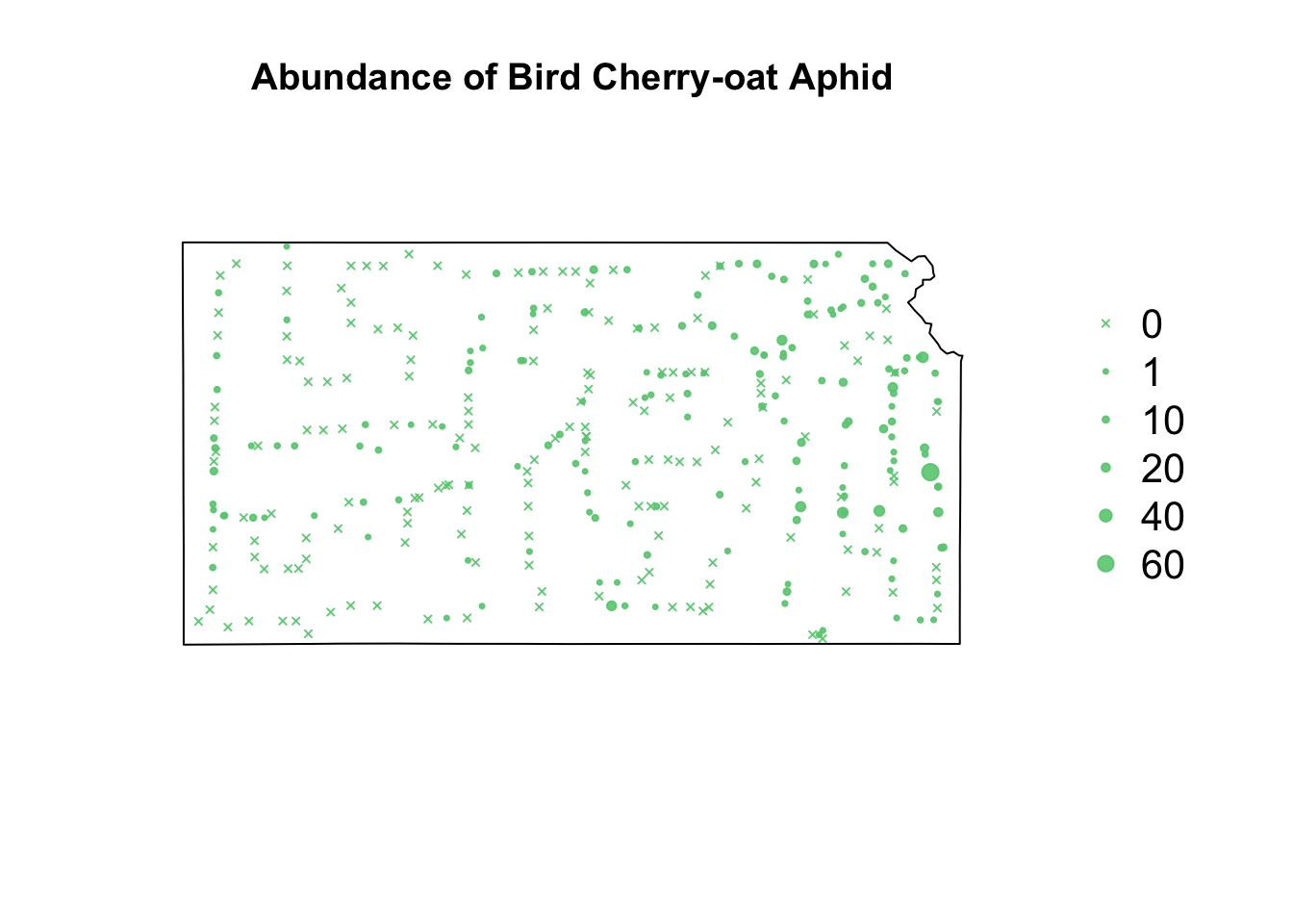
# Plot proportion of number of Bird cherry-oat aphid infected with BYDV
par(mar = c(5.1, 4.1, 4.1, 8.1), xpd = TRUE)
plot(sf.kansas, main = "Proportion infected")
points(pts.sample[, 4], col = rgb(0.8, 0.5, 0.4, 0.9), pch = ifelse(is.na(pts.sample$BYDV.prop) ==
    FALSE, 20, 4), cex = ifelse(is.na(pts.sample$BYDV.prop) == FALSE, pts.sample$BYDV.prop,
    0)/0.5 + 0.5)
legend("right", inset = c(-0.25, 0), legend = c("NA", 0, 0.25, 0.5, 0.75, 1), bty = "n",
    text.col = "black", pch = c(4, 20, 20, 20, 20, 20), cex = 1.3, pt.cex = c(0,
        0, 0.25, 0.5, 0.75, 1)/0.5 + 0.5, col = rgb(0.8, 0.5, 0.4, 0.9))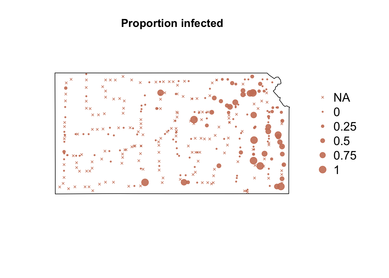
Study goals
- Make accurate predictions of vector abundance and probability of BYDV infection at times and locations where data was not collected.
- Understand the environmental factors (e.g., temperature) that influence the vector abundance and probability of BYDV infection.
Auxiliary data
- Weather/climate data
- Land cover data
- Crop data
Model choice: dynamic vs. descriptive spatio-temporal model?
- Class discussion
Next steps
- Write out the statistical model(s)
- Determine how we will evaluate how model(s)
- Determine how we will make inference